Machine learning
What backpropagation does before gradient descent takes a step
Work through backpropagation and a gradient descent update in matrix notation, with predictions, numerical gradients, dimension checks, and NumPy code.
In this article
![A batch with two examples, two features, and two outputs. Starting weights are the 2 by 2 identity and both biases are zero; loss is 1. Backpropagation computes a 2 by 2 weight gradient with every entry 1.5 and a bias gradient of (1, 1), without changing parameters. Gradient descent with learning rate 0.1 gives weights [[0.85, −0.15], [−0.15, 0.85]] and biases (−0.1, −0.1); new loss is 0.2025.](/visuals/journal/backprop-training-step.svg)
![A batch with two examples, two features, and two outputs. Starting weights are the 2 by 2 identity and both biases are zero; loss is 1. Backpropagation computes a 2 by 2 weight gradient with every entry 1.5 and a bias gradient of (1, 1), without changing parameters. Gradient descent with learning rate 0.1 gives weights [[0.85, −0.15], [−0.15, 0.85]] and biases (−0.1, −0.1); new loss is 0.2025.](/visuals/journal/backprop-training-step-dark.svg)
Two examples and two outputs: X = [[1, 2], [2, 1]], Y = [[0, 1], [1, 0]]. Predict with Ŷ = XW + 1bᵀ and divide the sum of squared residuals by 2m, with m = 2. Start at W = I and b = 0. Backpropagation leaves those parameters unchanged; gradient descent updates them using η = 0.1.
Original matrix worked example; values calculated from the batch and loss shown.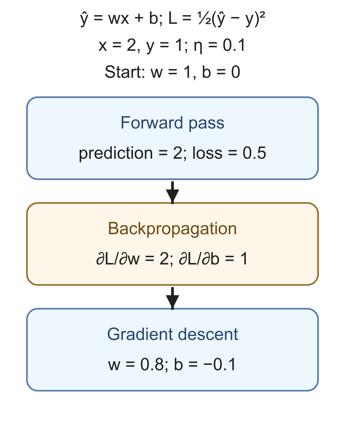
A typical PyTorch training loop calls loss.backward() and then optimizer.step(). You can stop between those calls and inspect the difference: the gradients have been calculated, while the parameters still have their old values.
Backpropagation computes the gradient of the loss with respect to each trainable parameter. Plain gradient descent uses those gradients to update the parameters. Other optimizers use different update rules, but occupy the same place in the PyTorch training loop, after the backward pass.
We will follow one batch through an affine layer using matrices throughout. Two examples, two input features, and two outputs keep the arithmetic small while showing how a batch produces a gradient for an entire weight matrix. The worked layer has no nonlinear activation; later, we connect its backward calculation to a multilayer network.
Start with a prediction and a loss
Put examples in the rows of an input matrix . For a batch of examples with input features and outputs, the prediction is
| Symbol | Shape | Meaning |
|---|---|---|
| One input example per row | ||
| Trainable weights | ||
| One trainable bias per output | ||
| A column of ones that repeats the bias across rows | ||
| Predictions and targets |
Every entry of is a separate parameter. For example, connects input feature 1 to output 2. All rows in the batch use the same and .
Here are our inputs and targets:
Start with an identity weight matrix and zero biases:
Multiplication by the identity leaves unchanged, so the predictions and residuals are
Use half the average squared error per example, summing over that example's outputs:
The squared Frobenius norm, , means square every entry and add. Here and all four residuals equal one, giving . The loss is a scalar even though its inputs and parameters are matrices. This normalization averages over examples, not over all matrix entries; the code below uses exactly this definition.
Work backward to find the gradients
Start at the loss. Its gradient with respect to the prediction matrix has one entry for every prediction:
Here is a partial derivative. It records how sensitive the loss is to prediction for example , holding the other prediction entries fixed.
For a scalar-valued loss, a gradient with respect to a matrix collects those partial derivatives in an array with the matrix's shape. Flattening that array gives the gradient vector for the flattened inputs. A Jacobian uses a different layout: one row per output and one column per input. The loss has just one output, so its Jacobian with respect to the flattened predictions would have one row; keeps the derivatives in the prediction matrix's original layout.
The backward pass through the affine layer gives
The matrix multiplication collects each example's contribution to every weight. In component form, . The bias derivative sums the incoming gradients over examples because the same bias was added to every row. Each gradient has the same shape as its parameter: for , and for .
For our batch,
For example, the derivative for is . Both examples contribute to that one parameter. The equal entries in these gradients come from the symmetric numbers chosen for this example; gradients in a trained network generally differ from entry to entry.
We have calculated six derivatives: four for the weights and two for the biases. The parameter matrices have not changed. Backpropagation has evaluated the chain rule through the graph. It has not chosen a learning rate or taken an optimization step. Our chain rule lesson explains the scalar case; the multivariable chain rule lesson shows how derivative matrices compose through intermediate values.
Use the gradients to update the parameters
The gradient descent update subtracts a scaled gradient from each parameter array. With learning rate ,
Using gives
Every derivative came from the same starting state. We calculate both gradients before changing either parameter array.
A new forward pass gives
Each prediction is now above its target. The new loss is , down from .
| Point in the calculation | Parameters changed? | Gradients available? | Loss at these parameters |
|---|---|---|---|
| After the forward pass | No | Not yet | 1 |
| After backpropagation | No | Yes | 1 |
| After gradient descent and a new forward pass | Yes | Gradients from the old state | 0.2025 |
The second row is the distinction you can inspect between loss.backward() and optimizer.step(). The backward pass adds derivative information; the optimization step changes the model.
For a classification loss, the starting derivative changes. Our cross-entropy derivative example derives the softmax logit gradient and checks it numerically. The same chain rule then carries that gradient through the network.
How this extends to a multilayer network
An affine layer inside a larger network still computes . Its incoming gradient now comes from the layers after it. Once that incoming gradient is known, the local backward rules remain
The last expression passes a gradient to the preceding layer when is itself a learned intermediate activation. Our vector–Jacobian product lesson explains how an incoming output sensitivity travels backward through a vector operation. These matrix formulas perform that same propagation while preserving the batch and feature axes.
If the affine layer is followed by an elementwise activation , the backward pass through that activation first computes , wherever the activation is differentiable. The symbol means entry-by-entry multiplication. Branches add contributions when multiple paths lead back to the same value. This is how the autograd computation graph organizes the chain rule across a network.
You may also see all weights and biases collected into one parameter vector . In that notation, the same plain gradient descent update is . Keeping separate matrices simply preserves the shapes of the layers.
Changing the learning rate does not change this starting gradient
Return to the original and , keep the same batch and loss, and choose . The starting gradients are unchanged. The larger update gives
Now every residual is , and the loss rises to . Even a direction that reduces the loss locally can make it worse if the step is too large.
For these starting matrices, each residual after one update is . The resulting loss is
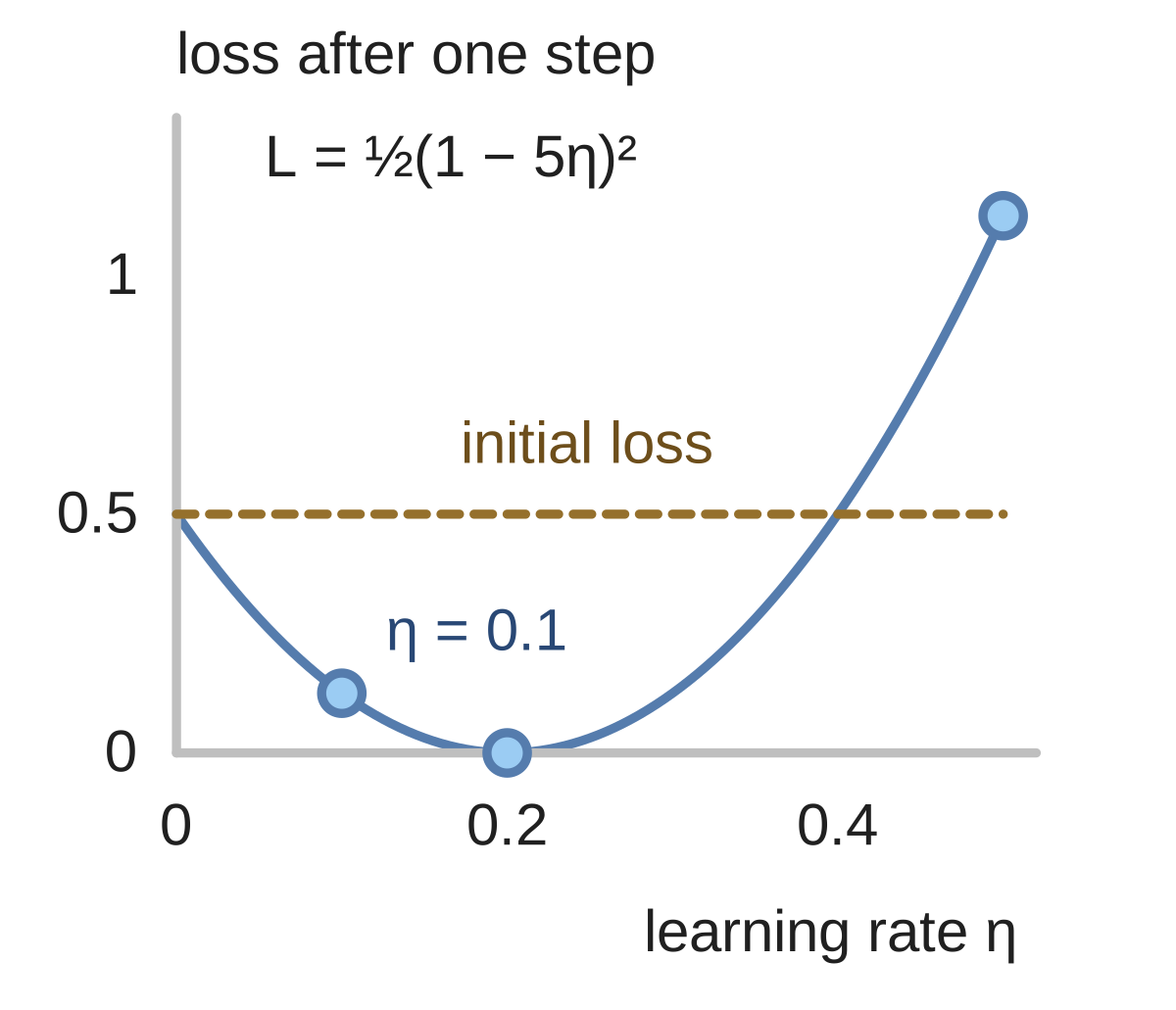
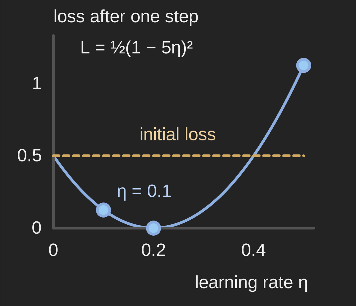
Every point starts from W = I and b = 0 on the same two-example batch and takes one matrix update. Only η changes. The minimum fits this illustrative batch exactly; it is not a recommended learning rate for other models.
Calculated from batch loss after one update = (1 − 5.5η)².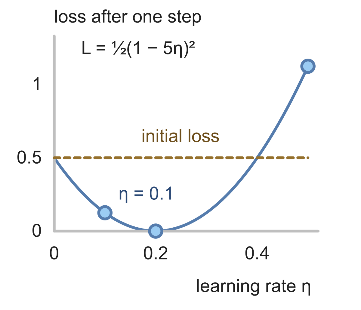
This plot varies one scalar, the learning rate, while the underlying update still changes all six parameters. The rate happens to fit this particular batch exactly. That is a consequence of our chosen numbers, not a recommended learning rate for a neural network. Our gradient descent oscillation article examines how step size affects repeated updates.
Reproduce the whole step in Python
The NumPy code below uses @ for matrix multiplication. b is stored as a column; adding b.T broadcasts the bias row across the batch. Both gradients are calculated before either parameter is updated.
import numpy as np

X = np.array([[1., 2.], [2., 1.]])
Y = np.array([[0., 1.], [1., 0.]])
W = np.eye(2)
b = np.zeros((2, 1))
m = X.shape[0]
eta = 0.1

# Forward pass: half the mean per-example squared error.
prediction = X @ W + b.T
residual = prediction - Y
loss = np.sum(residual ** 2) / (2 * m)

# Backward pass: each gradient matches its parameter's shape.
G = residual / m
grad_W = X.T @ G
grad_b = G.T @ np.ones((m, 1))

# Plain gradient descent uses gradients from the same state.
W_new = W - eta * grad_W
b_new = b - eta * grad_b
new_prediction = X @ W_new + b_new.T
new_loss = np.sum((new_prediction - Y) ** 2) / (2 * m)

print("weight gradient:\n", grad_W)
print("bias gradient:\n", grad_b)
print("new weights:\n", W_new)
print("new biases:\n", b_new)
print(f"loss: {loss:.4f} -> {new_loss:.4f}")
It prints the gradient and parameter matrices derived above, and loss: 1.0000 -> 0.2025. This code implements the local backward rules explicitly. In PyTorch, loss.backward() performs the differentiation and accumulates the results in parameter .grad attributes. A usual loop clears old gradients before the next backward pass unless it deliberately accumulates them across batches. The autograd tutorial explains that behavior.
What changes when you use a different optimizer?
The gradient calculation can stay the same when the update rule changes. SGD with momentum or Adam uses gradients together with optimizer state to determine an update. Its parameter changes therefore differ from the plain subtraction used in this article.
Gradient clipping adds another possible operation between the backward pass and the optimizer step. It limits the calculated gradients; the optimizer still determines how those gradients change the parameters.
When debugging, inspect the loss and computation graph if derivatives are wrong. If the derivatives are right but the loss grows after an update, examine the optimizer and step size. In our matrix example, changing only the learning rate was enough to turn an improving step into a harmful one.
Learn with Glacius
Want to go deeper into the math?
Build your understanding with visual lessons and practice on the concepts from this article.
Check the reasoning
Sources & notes
- PyTorch: Automatic Differentiation with torch.autograd ↗
Documents backward(), parameter gradients, and gradient accumulation.
- PyTorch: Optimizing Model Parameters ↗
Separates the backward pass from the optimizer update and explains the training loop.
Our figures use illustrative mathematical examples unless a dataset is explicitly identified. You can share the original Glacius figures with attribution and a link to this article; linked third-party material retains its own terms.
Keep exploring