Machine learning
Why gradient descent can oscillate
Why gradient descent oscillates: a visual, worked example showing convergence, overshooting, and divergence as the learning rate changes.
In this article
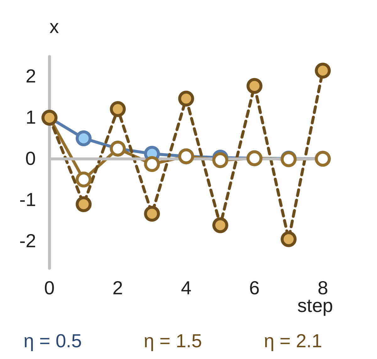
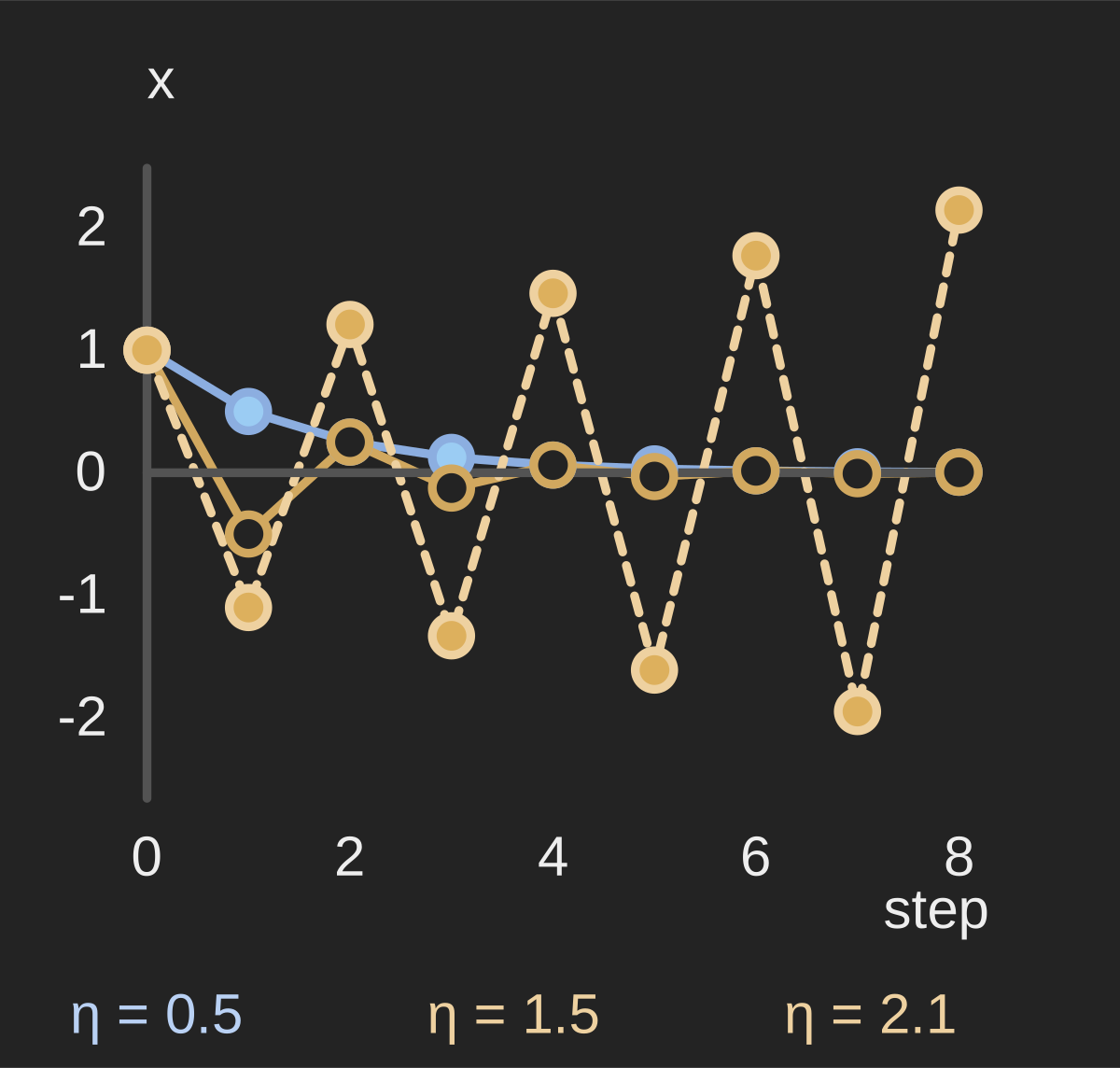
Filled markers: η = 0.5. Hollow markers: η = 1.5. Dashed line: η = 2.1. All start at x = 1 on the same quadratic.
Calculated from xₜ = (1 − η)ᵗ for f(x) = x²/2. Illustrative calculation, not training benchmark data.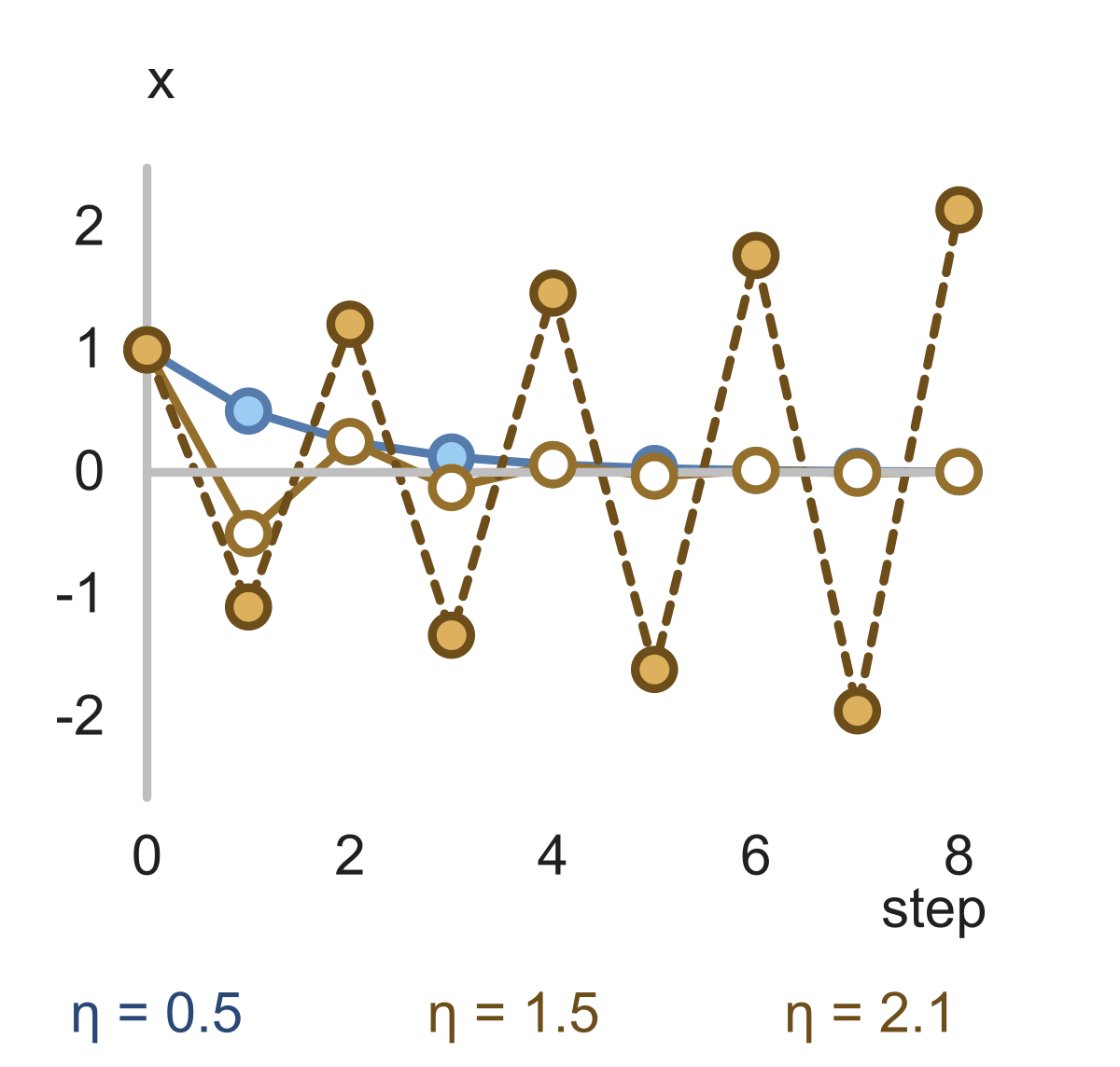
The gradient tells you which way a function increases locally. Taking a step in the opposite direction sounds like a reliable way to go downhill. So why can gradient descent bounce from one side of a minimum to the other—or get farther away?
A direction is not a step size. A locally useful direction can still carry you past the point you wanted to reach. A simple quadratic lets us calculate exactly when that happens.
A function we can see all the way through
Use . Its minimum is at , and its derivative is . Start at .
With a learning rate , gradient descent takes the update:
Each step multiplies the current value by the same number, . Repeating the update gives for our starting point. We can understand the whole trajectory by looking at that multiplier.
Three rates, three stories
With , the multiplier is 0.5. The sequence is . Each step closes half the remaining distance. The sign stays positive and the distance from zero gets smaller.
With , the multiplier is −0.5. Now the sequence is . Each step crosses the minimum. It oscillates, but its distance from zero still halves. This trajectory converges too.
With , the multiplier is −1.1. The sequence begins . It crosses zero and gets farther away every time. This one diverges.
The chart above plots the parameter against step number, rather than plotting the loss. That distinction matters: the parameter can oscillate even while the loss steadily falls.
| Learning rate | Multiplier | Parameter behavior |
|---|---|---|
| 0.5 | 0.5 | Approaches zero from one side |
| 1 | 0 | Reaches zero in one step |
| 1.5 | −0.5 | Oscillates toward zero |
| 2 | −1 | Alternates between 1 and −1 |
| 2.1 | −1.1 | Oscillates away from zero |
The exact boundary in this example
For the distance to zero to shrink, the magnitude of the multiplier must be less than 1:
Solving gives . Inside that interval, this quadratic converges from our starting point. At , it keeps bouncing at a fixed distance; above 2, the distance grows.
The threshold 2 belongs to this particular function. It is not a universal learning-rate recommendation. If we change the function to for , the derivative becomes , the multiplier becomes , and the convergence condition becomes .
Greater curvature reduces the size of a stable step. This is one reason a learning rate that works on one objective can fail on another.
What carries over to machine learning?
Real training problems can have many parameters, different curvatures in different directions, and noisy gradient estimates. The simple multiplier above no longer describes the full process.
But it gives you a useful question to ask when a training run behaves strangely: is the update direction wrong, or is the step too large for the local geometry? Dive into Deep Learning develops this idea further with examples of gradient descent.
Changing the learning rate is an experiment to evaluate, not a diagnosis by itself. Inspect the loss, check gradient calculations when appropriate, and compare runs under controlled conditions. A noisy curve can have more than one explanation.
Our backpropagation and gradient-descent example separates calculating the gradient from choosing the update. If you are considering a bound on unusually large gradients, the gradient-clipping comparison shows what norm and value caps change, including why bounded updates can still oscillate.
Predict the next step
For our original function, start again at and use . Where does the first update land? Does the next one cross zero?
Show the answer
The multiplier is . The first update lands at 0.2 and the second at 0.04. Neither crosses zero. Repeated updates approach zero from the positive side.
Continue with the step-size lesson, or revisit the gradient update to connect the formula to the direction of movement.
The figure’s downloadable CSV contains all nine plotted values for each rate, so you can reproduce the trajectories. These are exact-form calculations for an illustrative function, not measurements from a model-training benchmark.
Learn with Glacius
Want to go deeper into the math?
Build your understanding with visual lessons and practice on the concepts from this article.
Check the reasoning
Sources & notes
- Dive into Deep Learning: Gradient Descent ↗
Develops gradient descent in one and multiple dimensions and illustrates the effect of learning rate.
Our figures use illustrative mathematical examples unless a dataset is explicitly identified. You can share the original Glacius figures with attribution and a link to this article; linked third-party material retains its own terms.
Keep exploring
Lessons behind this article
- Gradient descent stepsCompute one gradient descent update.
- Learning ratesDiagnose overshooting from a step size on a one-dimensional quadratic.
- GradientsAssemble a gradient from partial derivatives in coordinate order.
- Stopping criteriaAssess a proposed stopping decision using gradient size and supplied tolerances.