Sample gradients

A sample gradient differentiates one selected example’s loss at the current parameter.

2 min read1 figureSources & further reading

On this page 8 sections

Overview
A model’s training loss combines errors from examples
For a vector parameter, prediction is w^T x
The residual alone omits the feature multiplier
A closer look
Key takeaway
Sources & further reading
Concept connections

01A model’s training loss combines errors from examples#

A model’s training loss combines errors from examples. A sample gradient measures one example’s contribution at the current parameter. Computing a small contribution can be much cheaper than processing a whole dataset, which is why stochastic training uses it.

Each example has its own loss and gradient at the current parameter. For one linear prediction with half-squared error:

\begin{gathered}\ell(w)=\tfrac12(wx-y)^2\\\ell\prime(w)=(wx-y)x\end{gathered}

With w=2, x=4 and y=3, prediction is 8 and residual is 5. Multiply that residual by the feature to get gradient 20.

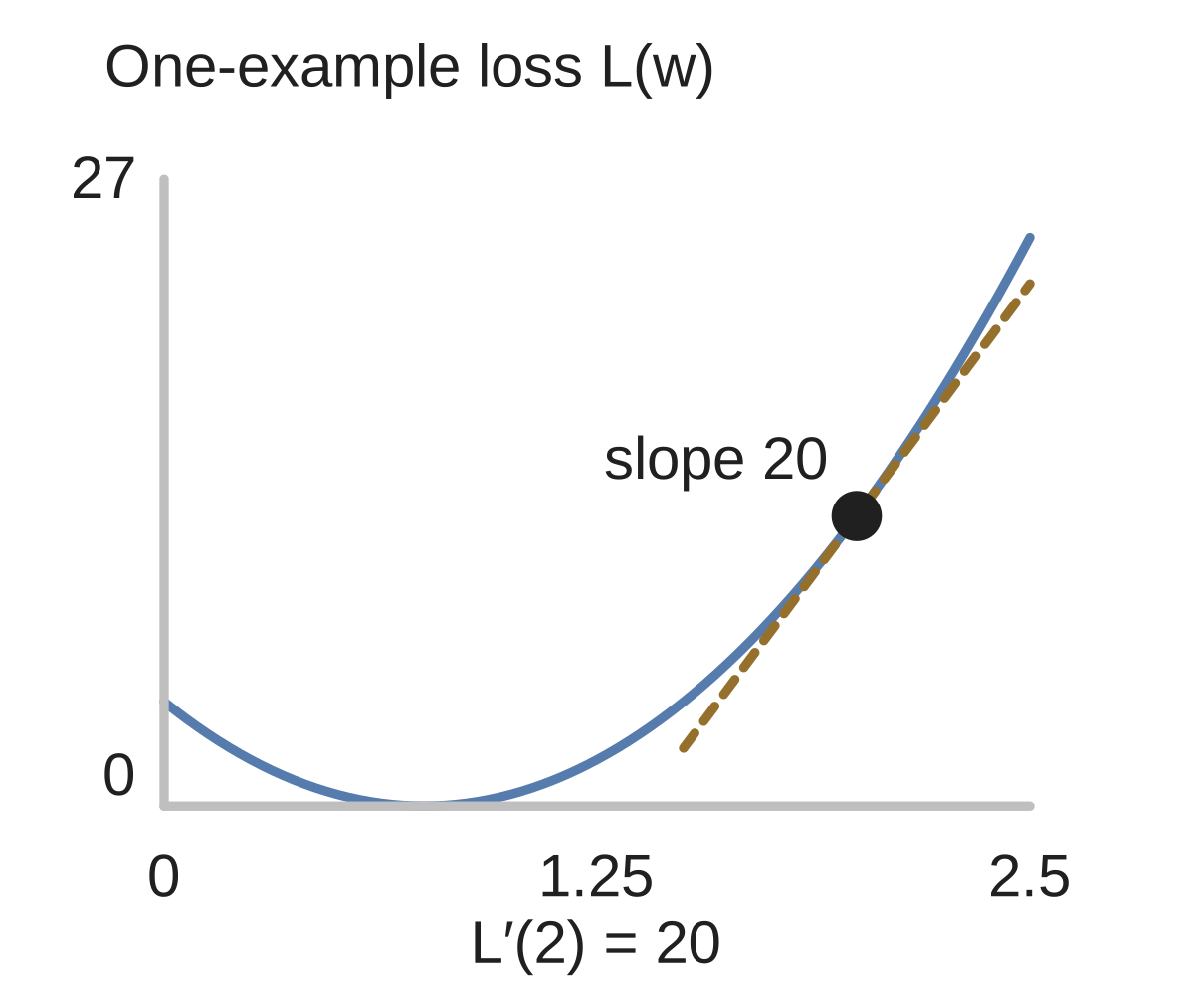
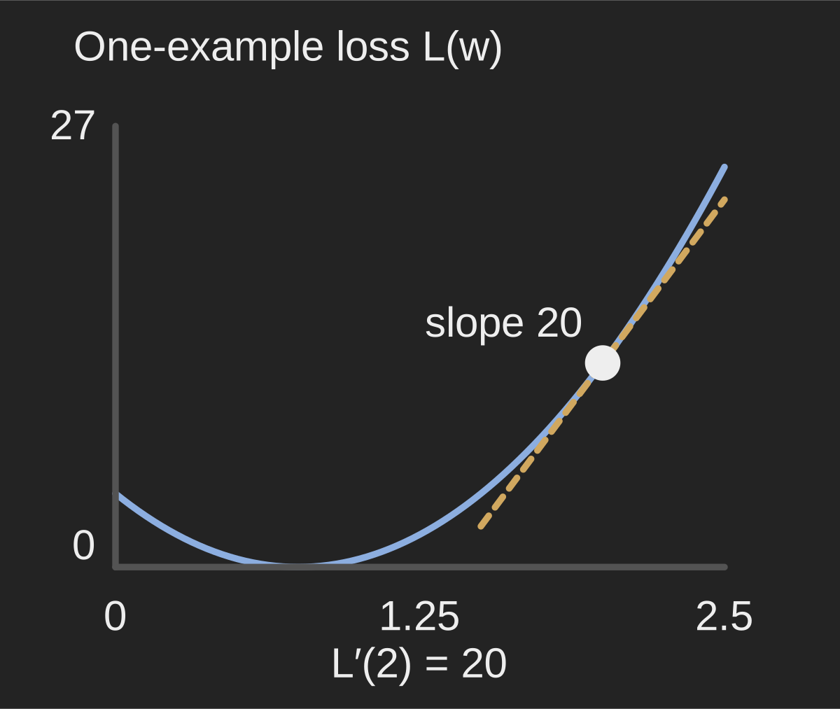
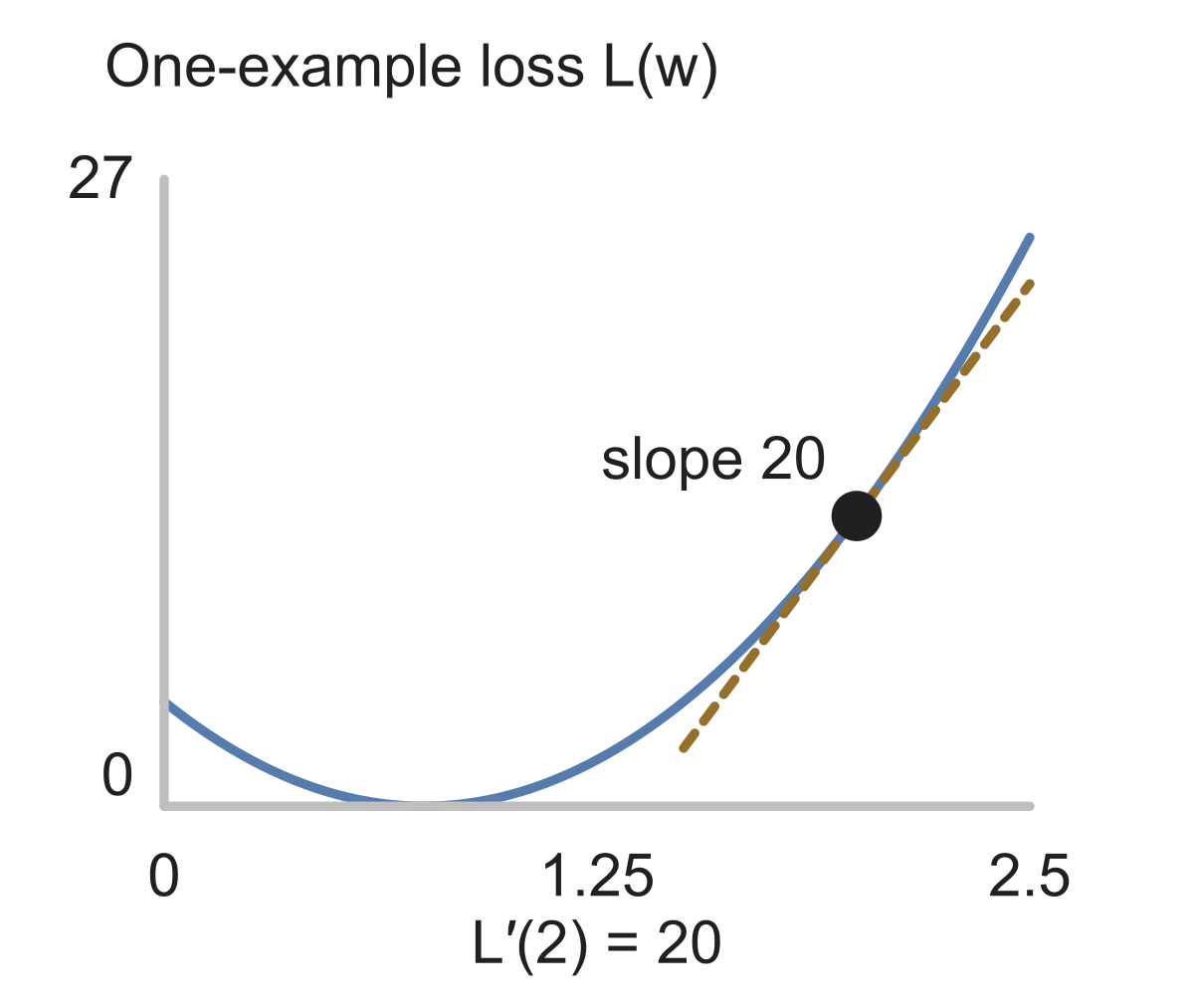
Figure 1For one example x=4,y=3, half-squared loss as a function of weight w is .5(4w−3)². At w=2, prediction is 8, residual 5, and loss 12.5. The tangent slope is residual times x = 20.

For prediction $wx$ and loss $\tfrac12(wx-y)^2$ , set residual $r=wx-y$ . The square contributes derivative $r$ with respect to the prediction; the prediction contributes derivative $x$ with respect to $w$ . Multiplying gives $rx$ . At $w=2,x=4,y=3$ , the residual is 5 and the gradient is 20.

Check your reasoning

Loss $\ell(w)=(wx-y)^2/2$ . Given $(w,x,y)=(3, -2, 1)$ , find $d\ell/dw$ .

Show answer and explanation

Residual -7 times feature -2 gives 14.

02For a vector parameter, prediction is w^T x#

For a vector parameter, prediction is $w^T x$ . The gradient of half-squared loss is $(w^T x-y)x$ .

Compute the residual once, then multiply every feature coordinate by it.

Check your reasoning

Half-squared loss, prediction $w^T x$ . Given $w=(2, 1)$ , $x=(1, 2)$ , $y=1$ . Find the gradient in w.

A $(3, 9)$
B $(3, 6)$
C $(4.5, 6)$

Show answer and explanation

$(3, 6)$

3×(1,2)=(3,6).

03The residual alone omits the feature multiplier#

The residual alone omits the feature multiplier. Its sign and magnitude can differ from the gradient.

A selected-example gradient can differ from the dataset average. Uniform sampling makes it unbiased for that average, not identical on every draw.

Check your reasoning

Loss $\ell(w)=(wx-y)^2/2$ ; $(w,x,y)=(1, 5, 2)$ . Draft gradient: $3$ . Correct it.

Show answer and explanation

Residual 3 times feature 5 gives 15.

04A closer look#

The residual and gradient are different: the feature value scales how much a weight change affects the prediction. An example with feature zero gives no gradient for that weight under this model, even if its prediction has a nonzero error.

Key takeaway

Differentiate the stated per-example loss; for half-squared linear error, multiply the residual by the feature.

Compute a single-example gradient for an empirical objective.

Sources & further reading

[1]
D2L §12.4.1, equations12.4.1–12.4.4 ↗D2L §12.4.1, equations12.4.1–12.4.4 · Article

01A model’s training loss combines errors from examples#

02For a vector parameter, prediction is w^T x#

03The residual alone omits the feature multiplier#

04A closer look#

Differentiate the stated per-example loss; for half-squared linear error, multiply the residual by the feature.

Sources & further reading

Reference this concept