Vector–Jacobian products

01Start with a scalar objective downstream#

Suppose a layer maps two inputs to two outputs: $y_1=2x_1+x_2$ and $y_2=3x_2$. Its output-row Jacobian is

Now a later computation assigns the scalar score $L=4y_1-y_2$. We want the rates of this score with respect to the layer's original inputs.

The score's output sensitivities are $\partial L/\partial y_1=4$ and $\partial L/\partial y_2=-1$. Collect them into a column $s=(4,-1)^T$.

These are rates, not the output values $(y_1,y_2)$. The incoming sensitivity says how a small change in each output would affect the scalar objective, after accounting for the computation downstream.

02Add the paths back to each input#

Input $x_1$ affects $y_1$ with rate $2$ and $y_2$ with rate $0$. Its total effect on $L$ is therefore $4(2)+(-1)(0)=8$.

Input $x_2$ affects both outputs, with rates $1$ and $3$. Its total effect is $4(1)+(-1)(3)=1$. The two paths partly cancel.

The resulting input gradient is $g=(8,1)^T$. The diagram places the incoming sensitivity at the top and the resulting input sensitivity below. The transposed Jacobian sits beside the arrow; we will unpack that matrix operation next.

Link to this figure ↗Download SVGDownload PNGCopy linkCopy embed

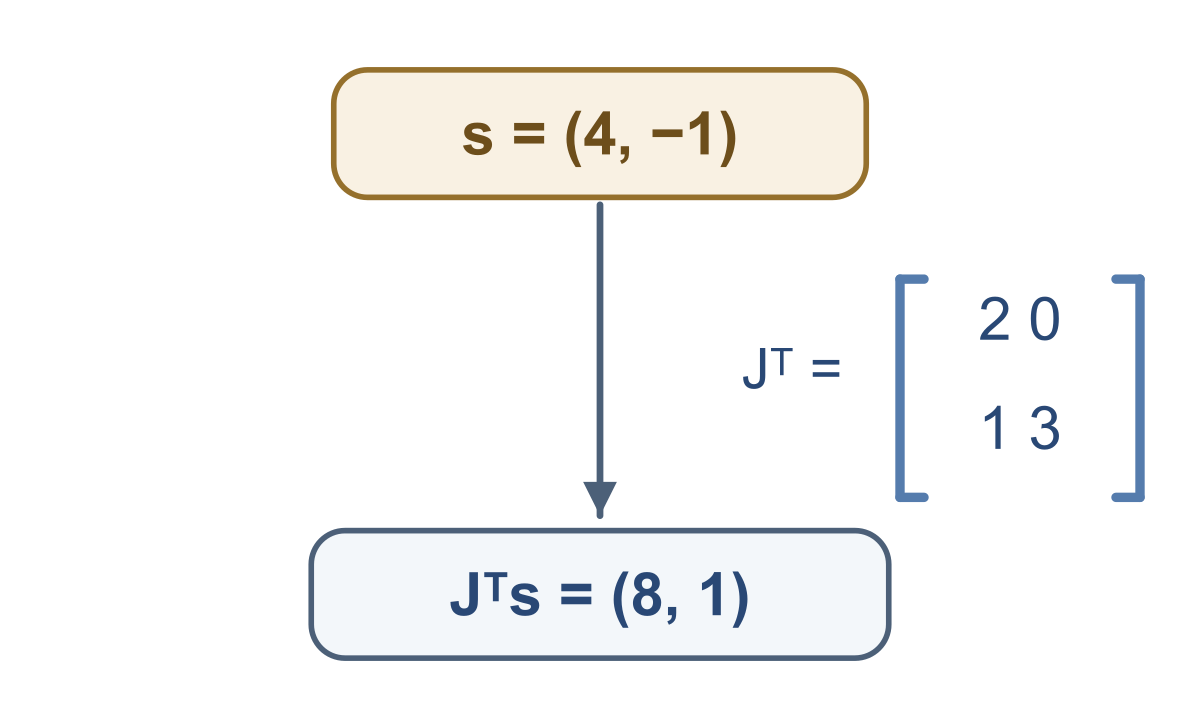
There is a direct check: substitute the layer's outputs into the score.

Its gradient with respect to the original inputs is $(8,1)^T$, matching the sum of path contributions. The local backward calculation recovered the derivative of the full composition.

03Read the vector–Jacobian product#

Using column gradients, the operation we just performed is

Each column of $J$ contains the effects of one input on all outputs. Transposing puts that column into a row, so its dot product with $s$ sums the contributions for that input.

The name “vector–Jacobian product,” or VJP, is often written using a row sensitivity: $s^TJ$. Its transpose is $J^Ts$, our column result.

The two forms contain the same derivatives. State the row or column convention before multiplying; the word “vector” by itself does not specify an orientation.

For a map with $n$ inputs and $m$ outputs, $J$ has shape $m\times n$. The incoming sensitivity $s$ has $m$ entries. Multiplying $J^T$, of shape $n\times m$, by $s$ returns $n$ input sensitivities.

This differs from $J\Delta x$, which sends an input perturbation forward to an output perturbation. A VJP sends sensitivities to a scalar objective backward.

04Apply a local backward rule#

For an elementwise square, $y_i=x_i^2$, each output depends only on the matching input. Its local derivative is $2x_i$, so the backward rule is

At $x=(2,-3)^T$ with incoming sensitivity $s=(5,2)^T$, the result is $g=(20,-12)^T$. The negative input produces a negative local derivative in the second coordinate.

The square map's Jacobian at this point is diagonal, with entries $4$ and $-6$. Multiplying its transpose by $s$ gives exactly the entrywise calculation above.

We do not need to allocate that full matrix to compute the result. A local rule can apply its effect directly, which is useful when a layer has many inputs and outputs.

05Check the orientation and accumulation#

In the first example, using $Js$ instead of $J^Ts$ gives $(7,-3)^T$. Both products happen to fit because $J$ is square, but only one collects all output paths for each input.

Check the meaning, not only the dimensions: the derivative for $x_2$ must include its influence on both $y_1$ and $y_2$. Those rates live in column two of $J$.

Across several layers, start from the final scalar objective and apply each local VJP in reverse order. Each local Jacobian is evaluated at the corresponding forward input.

When an intermediate value is used in more than one branch, add the incoming contributions from those branches before continuing backward. Replacing one contribution with another would discard a dependency path.

For matrix-shaped parameters, the resulting scalar-loss gradient can be arranged in the same shape as the parameter array. That arrangement preserves which derivative belongs to which parameter.

Computing these derivatives leaves the parameters unchanged. An optimizer then uses the gradients, together with its update rule and learning rate, to choose new parameter values.