Principal components
For centered observations stored as rows, principal directions are the right singular vectors ordered by singular value.
On this page 9 sections
01Understand the idea#
Principal component analysis, or PCA, finds new perpendicular feature directions that capture as much variation in centered observations as possible, one direction at a time. It is useful when many measured features move together and you want a smaller set of coordinates.
Imagine a cloud of centered two-feature observations stretched along a diagonal. The first principal direction follows its longest spread. The second is perpendicular and describes the remaining spread. A direction is a unit vector shared by all observations; each observation will get its own coordinate along it.
Put observations in the rows of and features in columns. In , the right singular vectors live in feature space, so they are the PCA directions. Larger singular values correspond to more variation along their paired directions. The factors are supplied in these tasks.
Put centered observations in the rows of . In its SVD, principal directions are the columns of . They live in feature space and are ordered by descending singular values.
With scales and rows , the first direction is column 1: . The second is .
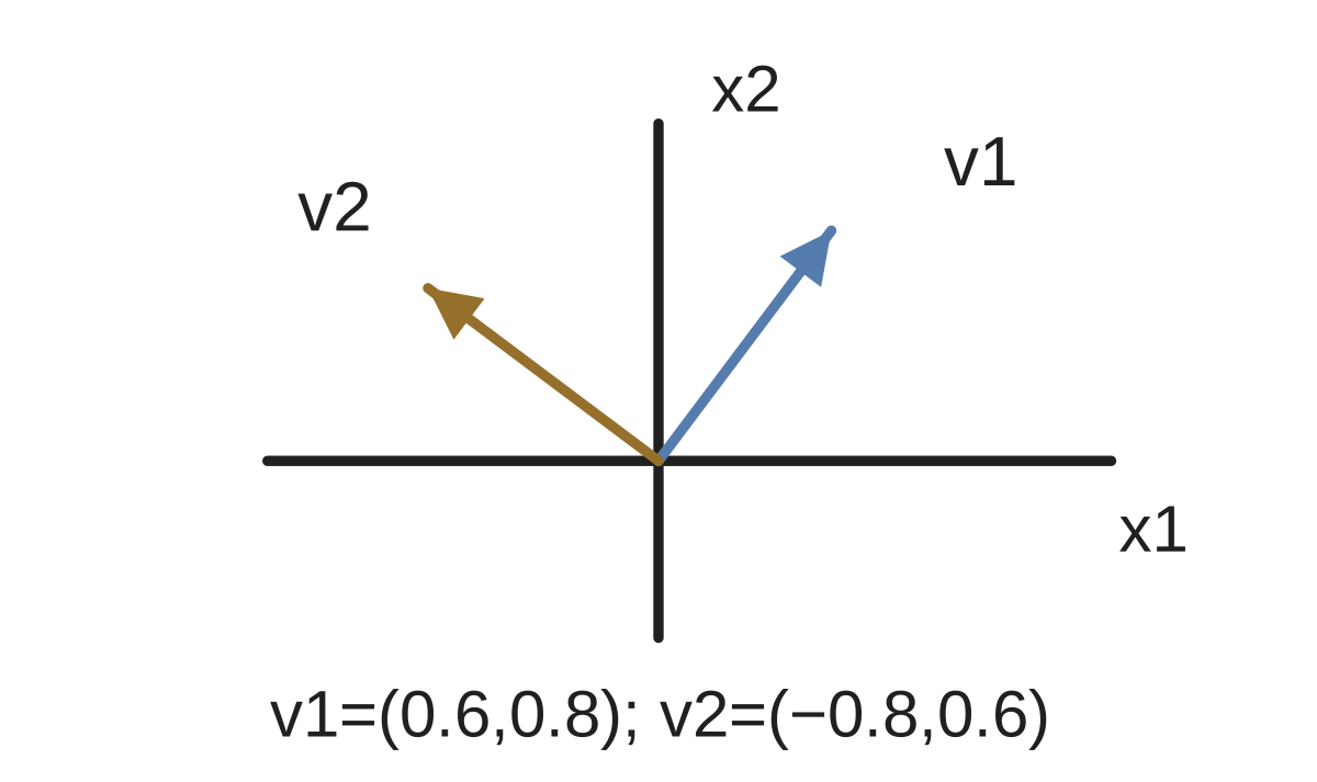
Read the matrix name before choosing entries. If has rows and , its first column is and its second is . Both have squared length 1. Multiplying the first by its scale 5 gives a stretched vector, not a unit principal direction.
Centered sample rows. SVD scales ; rows ; . Direction 1 (keep signs)?
Show answer and explanation
Column 1: .
02A closer look#
The singular scale describes spread along a direction; it does not multiply the unit direction. With distinct scales, reversing a direction’s sign changes its orientation but not its line. These tasks keep the supplied signs.
Centered sample rows. SVD scales ; rows ; . Claim: . Repair.
Show answer and explanation
Use unit column 1.
03When the factor is supplied as , use its rows#
When the factor is supplied as , use its rows. If has rows , those rows are the two principal directions in order. Do not take its columns again.
Transposition swaps rows and columns. If the supplied object is , each principal direction is already a row. Label it before extracting a vector. Direction 2 means the vector paired with the second singular value; it does not mean the second coordinate of direction 1.
Centered sample rows. SVD scales ; rows ; . Direction 2 (keep signs)?
Show answer and explanation
Row 2: .
04PCA can turn correlated sensor readings into fewer coordinates for plotting or modeling#
PCA can turn correlated sensor readings into fewer coordinates for plotting or modeling. It uses feature variation without target labels. A low-variance direction might still predict the target; a high-variance one may mostly reflect measurement units. Evaluate the reduced representation for its intended use.
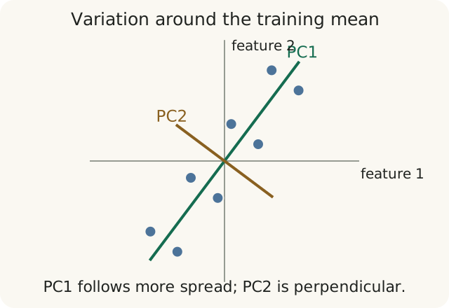
With observations as rows, use columns of V or rows of V-transpose. Keep each direction unit length and follow the singular-value order.
- Find principal directions from a supplied SVD of centered data.
Further questions
What if two singular values tie?
Sources & further reading
- [1]Cornell CS4780, Principal component analysis ↗Cornell CS4780 · Book