Singular value decomposition

01Singular value decomposition, or SVD, describes what a matrix does to vectors#

Singular value decomposition, or SVD, describes what a matrix does to vectors. A matrix may mix coordinates so its individual entries hide which directions it stretches or loses. SVD separates that action into a change of coordinates, a stretch along perpendicular axes, and a change to output coordinates.

Imagine a two-input sensor whose outputs mix both measurements. SVD finds perpendicular input directions that the sensor handles separately. Each has a matching output direction and a nonnegative stretch factor. A large factor means a strong response along that direction; a zero factor means that direction disappears.

The factorization is $A=U\Sigma V^T$. The columns of $V$ are input directions; $V^T$ measures a vector along them. The diagonal entries of $\Sigma$ are the singular values, written $\sigma_i$. The columns of $U$ are output directions. Here the factors are supplied: you will follow their action, rather than calculate a factorization from scratch.

Matrix products act on a vector from the right. First calculate $c=V^Tx$, then $d=\Sigma c$, then $y=Ud$. These are three different coordinate lists. Writing each one down prevents a common mistake: treating the scaled internal coordinates $d$ as the final output $y$.

In the example ahead, $V^T(a,b)=(b,-a)$ means “put the second input first, then negate the first.” For $x=(1,2)$, substitute $a=1,b=2$, giving $c=(2,-1)$. The letters $a,b$ are placeholders; use the newest pair at every stage.

Start $A=U\Sigma V^T$ with $V^T$. It gives right-singular coordinates. For $x=(1,2)$ and $V^T(a,b)=(b,-a)$, these are $(2,-1)$.

Link to this figure ↗Download SVGDownload PNGCopy linkCopy embed

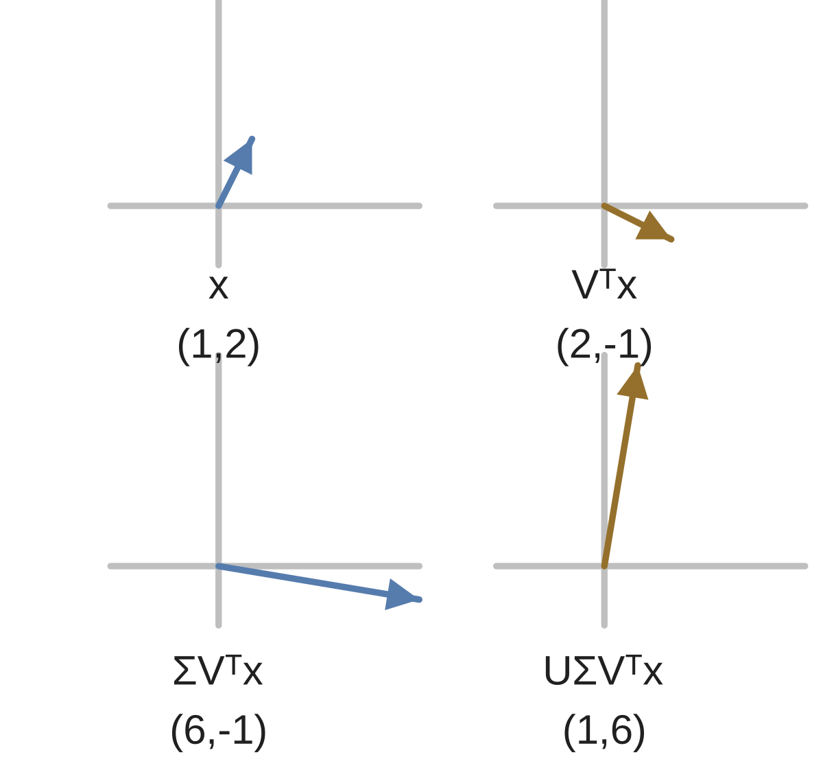
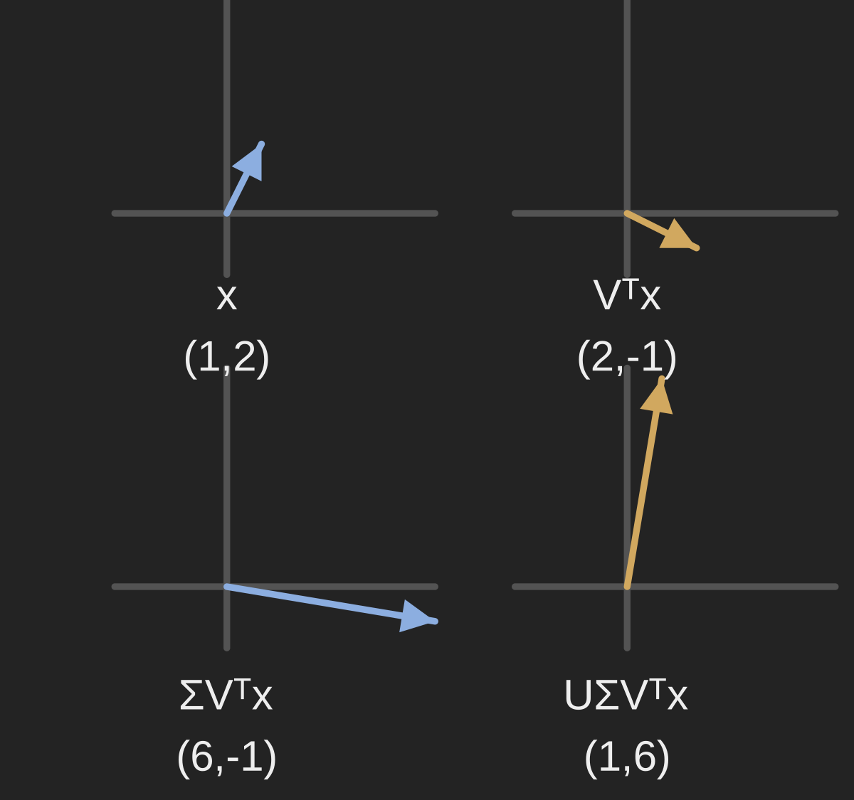
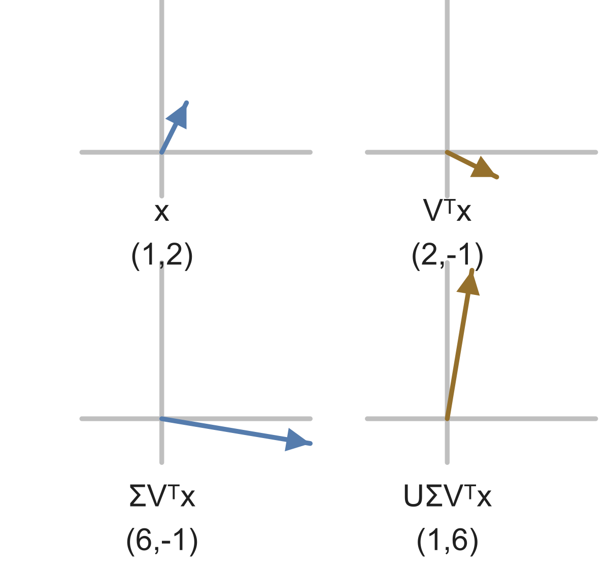
Continue with right coordinates $(2,-1)$. Scales $(3,1)$ give $(6,-1)$. Then $U(a,b)=(-b,a)$ turns those into output $(1,6)$.

Follow the complete example again: $x=(1,2)$ becomes $c=(2,-1)$. Scaling by $(3,1)$ gives $d=(3\times2,1\times(-1))=(6,-1)$. Finally $U(a,b)=(-b,a)$ gives $y=(-(-1),6)=(1,6)$. Each factor consumes the previous result, never the original input again.

02U and V are orthogonal: they preserve lengths and angles, and may rotate or reflect#

$U$ and $V$ are orthogonal: they preserve lengths and angles, and may rotate or reflect. $\Sigma$ scales along coordinate axes; a zero scale erases that coordinate. Apply these actions in their supplied order.

03Sometimes a problem gives the output basis columns instead of an action rule#

Sometimes a problem gives the output basis columns instead of an action rule. If $U$ has columns $u_1,u_2$, then $U(d_1,d_2)=d_1u_1+d_2u_2$. Multiply each entire column by its matching coefficient, then add matching entries. This is the column-combination view of matrix multiplication you already learned.

For $c=(1,-2)$ and singular values $(4,1)$, first get $d=(4,-2)$. With $u_1=(0,1)$ and $u_2=(-1,0)$, the contributions are $4u_1=(0,4)$ and $-2u_2=(2,0)$. Adding gives $(2,4)$. The pair $(4,-2)$ was a pair of weights, not the answer in the original output axes.

Right coordinates can be supplied directly. For $c=(1,-2)$, scales $(4,1)$ give $(4,-2)$. With $u_1=(0,1)$ and $u_2=(-1,0)$, return to output coordinates by combining these basis vectors.

04A closer look#

In a data matrix, this separation lets us describe strong patterns with a few direction pairs. Later lessons keep the largest components to compress a matrix and use input directions to build PCA features. Reading the three factors now makes those methods interpretable instead of turning them into unexplained formulas.

The small problems use square, two-dimensional factors so every step is visible. SVD also works for rectangular matrices: the input and output spaces can have different sizes. A full real factorization of an $m\times n$ matrix uses $V^T$ of size $n\times n$, $\Sigma$ of size $m\times n$, and $U$ of size $m\times m$.

Further questions