Machine learning
The cross-entropy derivative, one logit at a time
Derive softmax cross-entropy with respect to logits, check p − y with a three-class example, and see what changes with soft labels, weights, and batch means.
In this article
- A three-class prediction you can calculate by hand
- Derive the gradient by writing the loss in logits
- Why the derivative with respect to probability is different
- Read the derivative as a local change in loss
- Verify the calculation with stable Python
- Soft labels, class weights, and batch means
- Match the formula to the loss you actually call
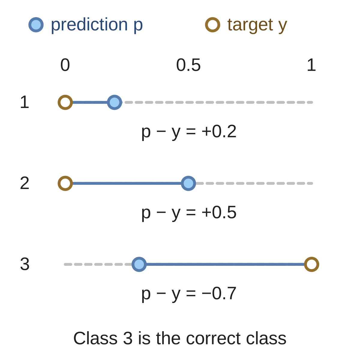
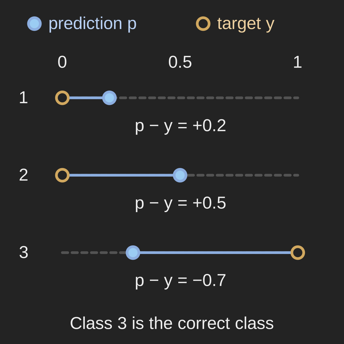
One illustrative example: logits z = (ln 2, ln 5, ln 3) produce p = (0.2, 0.5, 0.3), and the target is class 3. Filled markers show predictions; hollow markers show targets. Horizontal distances use one probability scale. The signed gaps are the logit derivatives for unweighted cross-entropy with natural logarithms.
Original calculation from the displayed logits and target; not measured classification results.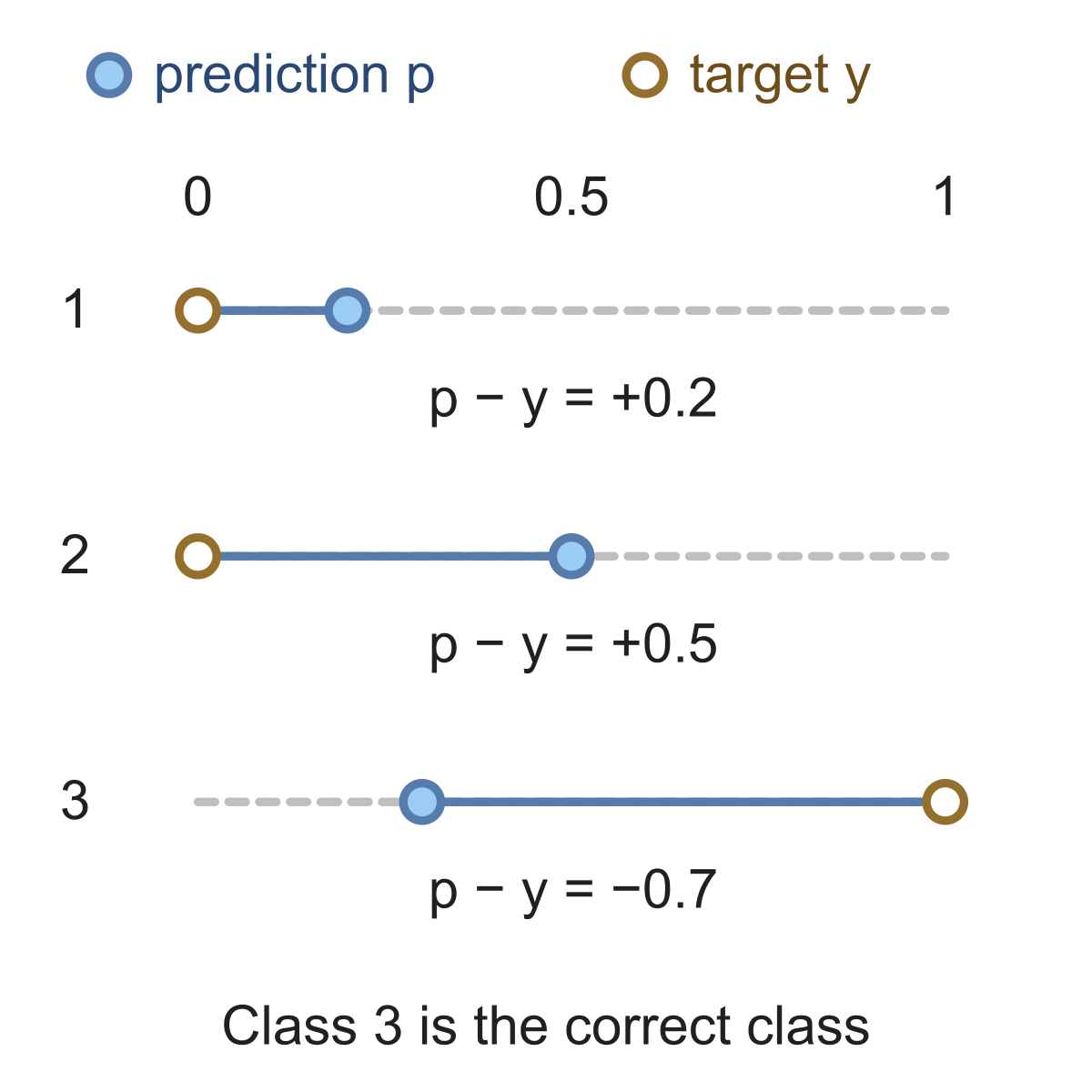
Suppose a classifier gives the correct class a probability of . Its cross-entropy loss is . Differentiate that loss with respect to the probability and you get . Differentiate it with respect to the logit that produced the probability and you get .
Both derivatives are correct. They describe changes to different inputs. The familiar cross-entropy gradient is with respect to logits, after composing the loss with softmax. For one unweighted example, natural logarithms, and a fixed target distribution that sums to one,
We will calculate those derivatives for three classes, work through why every logit matters, and check the result by perturbing the inputs in Python.
A three-class prediction you can calculate by hand
A logit is a real-valued score before softmax converts the scores into probabilities. Choose
The target is class 3. Using logarithms for our starting scores makes the exponentials easy to check:
The prediction favors class 2 even though the target is class 3. For fixed targets , categorical cross-entropy is
With our one-hot target, only the third term contributes: . The cross-entropy lesson explains this loss as the cost of assigning probability to outcomes; here we are interested in its sensitivity to the model's scores.
Subtract the target from the prediction one entry at a time:
| Class | Probability | Target | Logit derivative |
|---|---|---|---|
| 1 | 0.2 | 0 | 0.2 |
| 2 | 0.5 | 0 | 0.5 |
| 3 | 0.3 | 1 | −0.7 |
The positive derivatives mean that increasing either wrong-class logit raises the loss locally. The negative derivative for class 3 means increasing that logit lowers it. Gradient descent subtracts the gradient, so a direct update to these scores would lower the first two and raise the third.
Derive the gradient by writing the loss in logits
The shortest route avoids a full softmax Jacobian. Take the logarithm of the probability:
Substituting into the loss gives two terms:
Because the targets sum to one, this becomes
When we differentiate with respect to , the log-sum-exp term contributes . The target-weighted sum contributes . Therefore
This is the same calculation developed in Dive into Deep Learning's softmax regression chapter. The result uses the whole probability distribution: changing one logit changes the denominator shared by every class.
Why the derivative with respect to probability is different
Before passing through softmax, the loss has partial derivatives
This treats the positive coordinates of as separate inputs to the loss expression. The softmax operation then accounts for how those coordinates move together. For our example, the incoming gradient with respect to probabilities is .
The softmax Jacobian contains a derivative for each output probability with respect to each input logit:
Here is one when and zero otherwise. Increasing a class's own logit increases its probability at rate ; increasing another class's logit decreases it at rate .
Only contributes directly to our one-hot loss. Its derivatives with respect to all three logits are
Multiplying by yields again. The wrong classes have nonzero logit gradients because both affect through softmax's denominator.
For a general normalized target, the multivariable chain rule sums all those paths:
Multiplying by the softmax derivative a second time would differentiate through softmax twice. Once you have , you already have the gradient at the logits.
Read the derivative as a local change in loss
Hold and fixed, and vary only the correct-class logit . The loss becomes a function of one number:
At , its slope is . Increasing this logit by a small amount changes the loss by approximately . For example, predicts a change of ; the exact change is about .
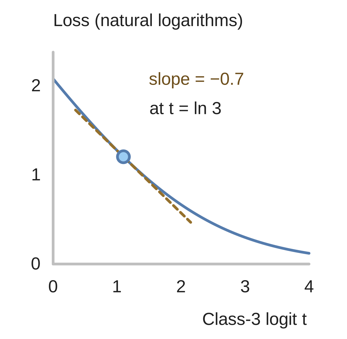
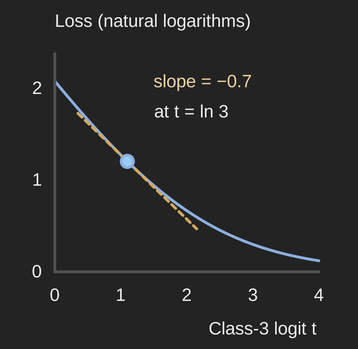
Hold z₁ = ln 2 and z₂ = ln 5 fixed, and vary z₃ = t. The solid curve is L(t) = ln(7 + eᵗ) − t. The point marks t = ln 3 and loss ≈ 1.204. The dashed tangent has slope −0.7; increasing t by 0.01 lowers loss by approximately 0.006989.
Original one-coordinate calculation using the same three-class example and natural-log loss.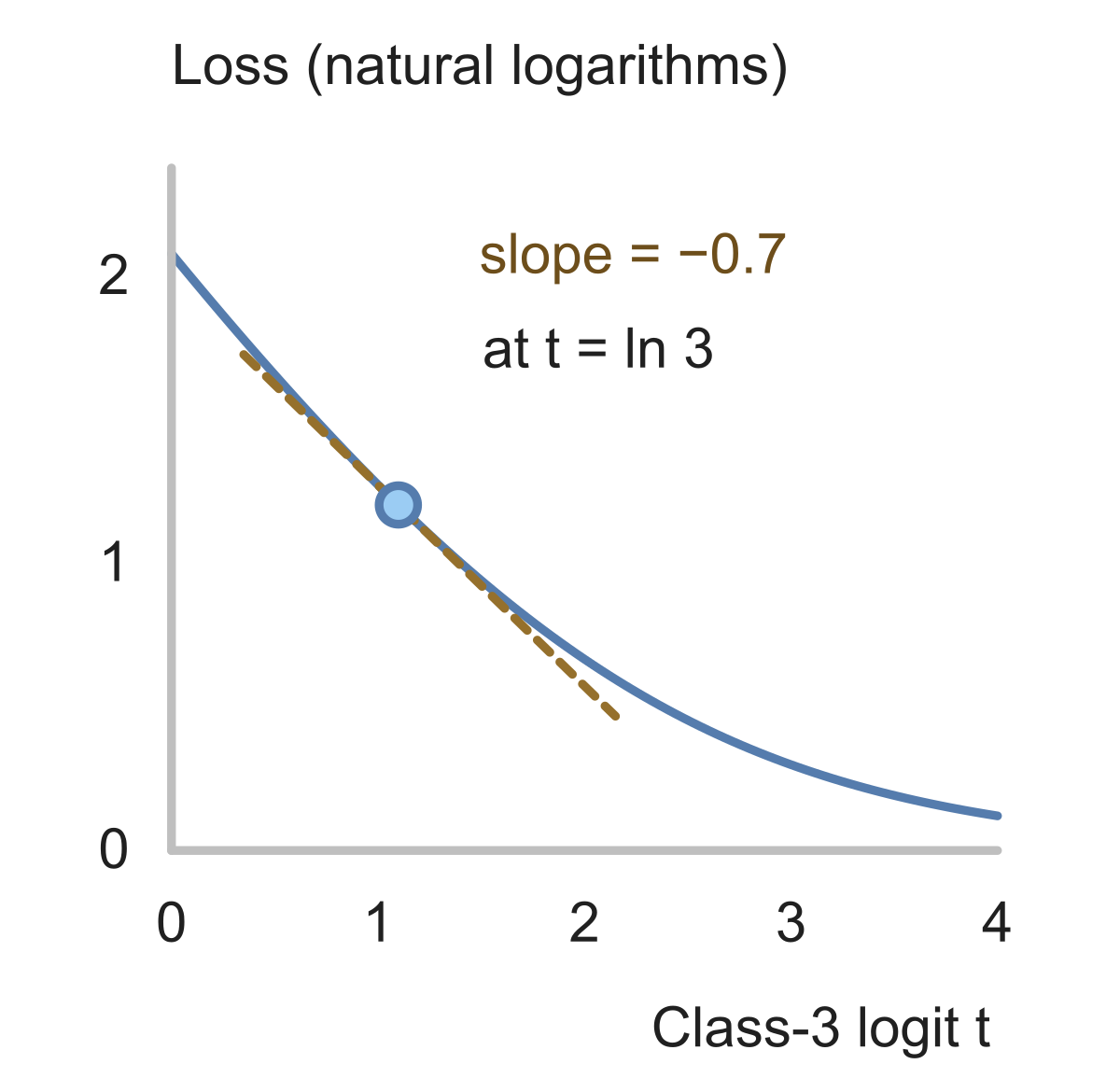
The tangent describes the nearby curve. Farther away, the probability changes and so does the derivative. The other two logits also have their own positive slopes at the starting point; this plot isolates the third coordinate rather than showing a full training trajectory.
As another check, the three logit derivatives sum to zero. Adding the same constant to every logit leaves softmax unchanged, so it must leave the loss unchanged as well.
Verify the calculation with stable Python
This example uses only Python's standard library. Subtracting the largest logit keeps the exponentials at or below one. Computing the loss from the shifted logits avoids taking the logarithm of a probability that may have rounded to zero.
import math


def cross_entropy(logits, target):
    if not logits or len(logits) != len(target):
        raise ValueError("Use equal, nonempty vectors")
    if not all(math.isfinite(v) for v in [*logits, *target]):
        raise ValueError("Inputs must be finite")
    if any(v < 0 for v in target) or not math.isclose(
        math.fsum(target), 1.0, rel_tol=0, abs_tol=1e-12
    ):
        raise ValueError("Target must be a probability distribution")

    largest = max(logits)
    shifted = [v - largest for v in logits]
    exponentials = [math.exp(v) for v in shifted]
    total = math.fsum(exponentials)
    probabilities = [v / total for v in exponentials]
    loss = math.log(total) - math.fsum(
        y * z for y, z in zip(target, shifted)
    )
    gradient = [p - y for p, y in zip(probabilities, target)]
    return loss, probabilities, gradient


z = [math.log(2), math.log(5), math.log(3)]
y = [0.0, 0.0, 1.0]
loss, p, gradient = cross_entropy(z, y)

# Central differences perturb one logit while fixing the others.
h = 1e-5
numeric = []
for j in range(len(z)):
    plus, minus = z.copy(), z.copy()
    plus[j] += h
    minus[j] -= h
    numeric.append(
        (cross_entropy(plus, y)[0] - cross_entropy(minus, y)[0])
        / (2 * h)
    )

assert max(abs(a - b) for a, b in zip(gradient, numeric)) < 1e-8
print("probabilities:", [round(v, 6) for v in p])
print("analytic:", [round(v, 6) for v in gradient])
print("numeric: ", [round(v, 6) for v in numeric])
print(f"loss: {loss:.6f}")

# A direct step in logit space, not a network parameter update.
new_z = [v - 0.5 * g for v, g in zip(z, gradient)]
print(f"loss after step: {cross_entropy(new_z, y)[0]:.6f}")
Both gradient lines print [0.2, 0.5, -0.7]. The loss changes from 1.203973 to 0.850053 after the direct logit update. The finite-difference check estimates each derivative using only evaluations of the loss, independently of the expression.
In a neural network, the logits depend on weights and earlier activations. Backpropagation carries this gradient through those operations to the parameters before the optimizer takes a step. Our backpropagation and gradient descent example follows that process through an affine layer. Its squared-error loss has a different starting derivative; the same chain-rule machinery carries it backward.
Soft labels, class weights, and batch means
Soft labels still give p minus y
Nothing in the derivation required a single entry of to equal one. It required , with the targets held fixed while differentiating the logits. If our target becomes , the gradient at the same prediction is .
For label smoothing, substitute the actual smoothed target into . Do not keep subtracting the original one-hot vector. TensorFlow's softmax cross-entropy documentation likewise requires each label vector to form a valid probability distribution.
Class weights change the expression
If the per-example loss is instead
the same differentiation gives
For a one-hot target in class , this simplifies to : the target class's weight scales the entire gradient. For soft targets, multiplying each entry of by its own class weight generally gives the wrong answer.
For instance, use and soft target . Then , and the weighted gradient at is . It still sums to zero.
A mean introduces a denominator
For an unweighted batch of examples with , the derivative for row is . A summed loss has no factor. This assumes each row contributes one classification loss and none are ignored.
Framework reductions deserve a check when using weights. PyTorch's weighted mean with class-index targets divides by the sum of the non-ignored target weights. With probability targets, its mean divides by the number of loss elements. These denominators can produce different gradient scales even when the unreduced losses match. See the explicit formulas in PyTorch's CrossEntropyLoss reference.
Match the formula to the loss you actually call
PyTorch's CrossEntropyLoss and TensorFlow's softmax_cross_entropy_with_logits accept logits and perform the required normalization internally. Passing softmax probabilities as their logit input changes the function being optimized. TensorFlow documents this input requirement explicitly.
For binary classification with one sigmoid output, the analogous result is also with respect to its logit. The probability derivative differs: for , it is . The sigmoid derivative supplies the cancelling factor . Independent sigmoid outputs for multilabel classification therefore need their own loss setup, rather than one softmax across all labels.
All calculations here use natural logarithms. A base-two loss and its derivatives are larger by . When checking a mismatch in your own implementation, first identify the differentiated variable, the target distribution, and the reduction. The short expression is useful precisely because those choices are explicit.
Learn with Glacius
Want to go deeper into the math?
Build your understanding with visual lessons and practice on the concepts from this article.
Check the reasoning
Sources & notes
- Dive into Deep Learning: Softmax Regression ↗
Defines softmax and cross-entropy and derives the gradient with respect to logits.
- PyTorch 2.11: CrossEntropyLoss ↗
Specifies logit inputs, class weights, target formats, label smoothing, and reduction denominators.
- TensorFlow: softmax_cross_entropy_with_logits ↗
Documents normalized label distributions and the requirement to pass logits rather than softmax outputs.
Our figures use illustrative mathematical examples unless a dataset is explicitly identified. You can share the original Glacius figures with attribution and a link to this article; linked third-party material retains its own terms.
Keep exploring
Lessons behind this article
- Cross-entropyCompute expected negative log probability under a supplied target distribution.
- JacobiansConstruct the Jacobian of a vector-valued map.
- Gradient checksDiagnose a mismatch between analytic and numerical derivatives using a stated tolerance.
- Multivariable chain ruleCompute the derivative of a composed vector map using Jacobians.