Local linearization

01Use a tangent as a local model#

Local linearization estimates a nearby function value from a known value and derivative. The derivative converts a small input change into an estimated output change.

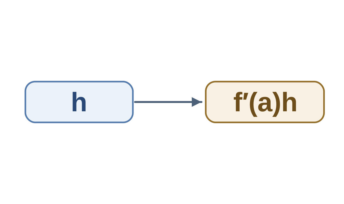
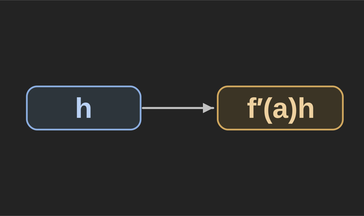
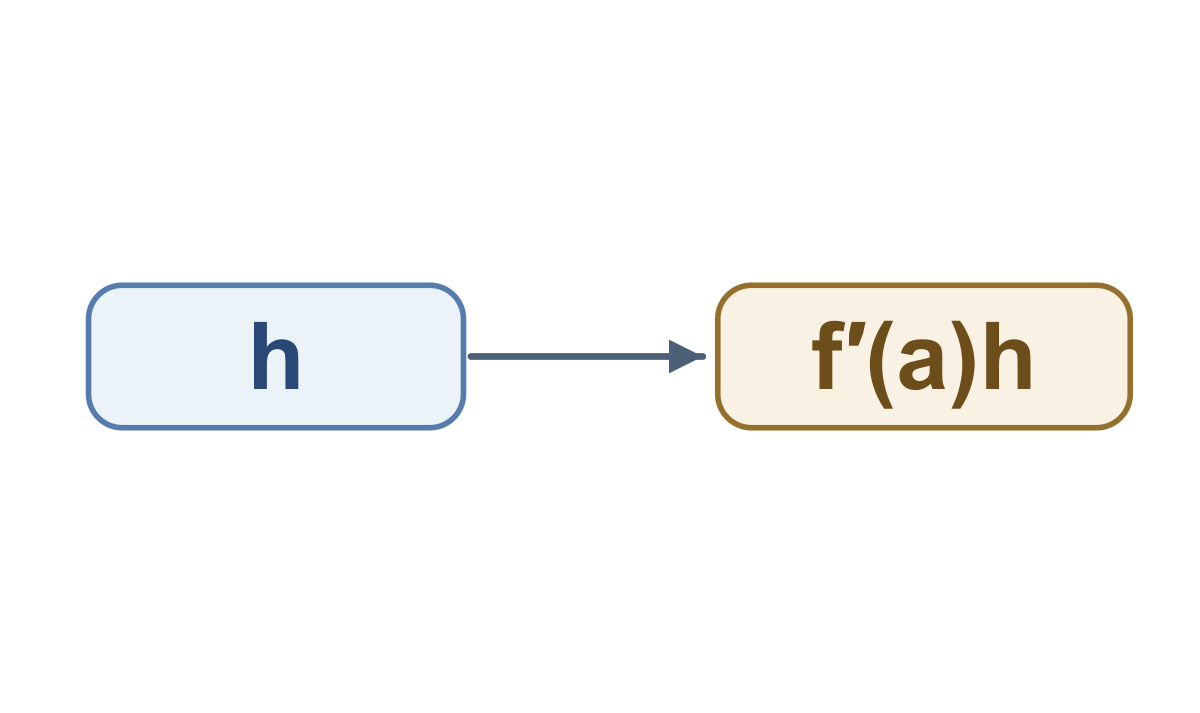
At base input $a$, let the displacement be $h$. The tangent gives

The derivative multiplies the displacement $h$, not the final input $a+h$.

02Estimate and compare#

For $f(x)=x^2$, use $a=2$, $f(2)=4$, and $f'(2)=4$. To estimate $f(2.1)$, the input change is $0.1$. The estimated output change is $4(0.1)=0.4$, giving $4.4$.

The exact value is $2.1^2=4.41$. Expanding $(2+h)^2$ gives $4+4h+h^2$. The linearization keeps the constant and linear terms; here the omitted term is $h^2=0.01$.

03Direction, size, and limits#

A negative displacement uses the same rule. At $a=2$, a displacement of $-0.1$ gives an estimate of $4-0.4=3.6$, compared with the exact value $3.61$.

For a differentiable function, the approximation error becomes small relative to the input displacement as the displacement approaches zero. This does not promise accuracy for a large step. At input $3$, the same linear model estimates $8$ while the square is $9$.

The approximation is exact for an affine function because there is no curvature term. In optimization, local linear models help predict what a small parameter change will do; checking a finite step still matters.