Expected transformed values
E[g(X)] is the probability-weighted sum of g(x) over possible values x.
On this page 7 sections
01To find the expected value of a function , apply to each possible value first#
To find the expected value of a function , apply to each possible value first. Keep its original probability as the weight.
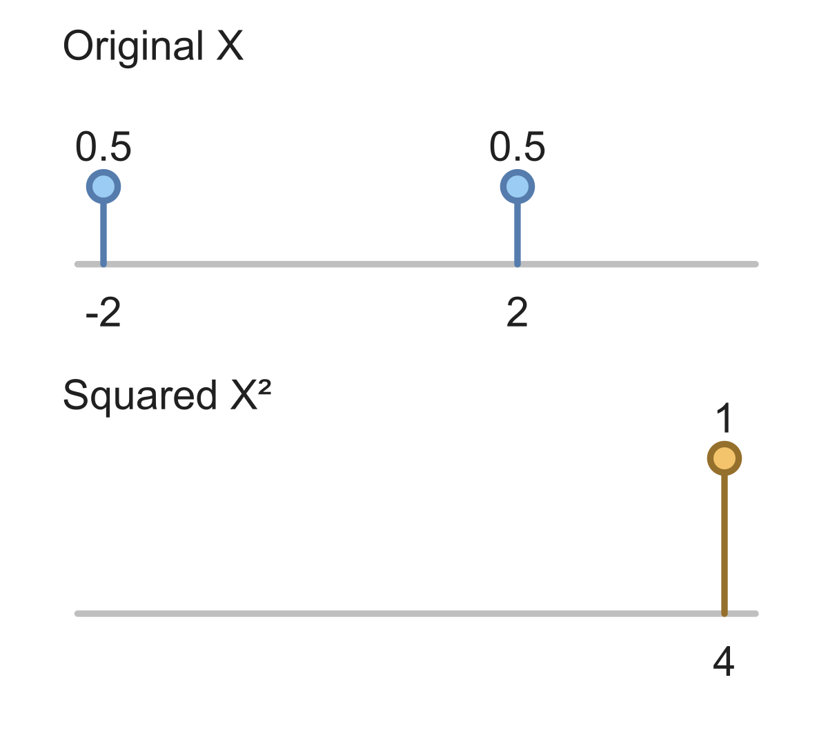
If is equally likely to be or , both values square to , giving .
![X is −2 or 2 with probability 1/2 each. The top number line carries those masses. Under squaring both outcomes map to 4, so the lower transformed distribution has all mass at 4. Thus E[X²]=4, while E[X]=0.](/visuals/p-lotus/comparison-1gj5720.svg)
![X is −2 or 2 with probability 1/2 each. The top number line carries those masses. Under squaring both outcomes map to 4, so the lower transformed distribution has all mass at 4. Thus E[X²]=4, while E[X]=0.](/visuals/p-lotus/comparison-1gj5720-dark.svg)
PMF: , . Find .
Show answer and explanation
Transformed values: . Weighted sum: .
02The same procedure works for a supplied cost rule#
The same procedure works for a supplied cost rule. If , compute each cost , multiply by , and sum.
You can work directly from the original distribution; a separate probability table for the transformed values is optional.
PMF: , . Cost is . Find .
Show answer and explanation
Transformed values: . Weighted sum: .
03In the example, , so #
In the example, , so . But . Squaring and averaging give different results when their order is swapped.
For a nonlinear function, transform each possible value before you average.
PMF: , . A learner uses . Repair the calculation of .
Show answer and explanation
Transformed values: . Weighted sum: .
Apply the function to each value before taking the weighted average.
- Compute the expectation of a function of a discrete random variable.
Sources & further reading
- [1]Pishro-Nik, Introduction to Probability: Functions of Random Variables ↗Pishro-Nik: Introduction to Probability · Article