Probability calibration
Calibration compares predicted probabilities with observed positive frequencies in comparable groups.
On this page 8 sections
01Understand the idea#
A probability model is calibrated when groups of predictions near a given probability show the event about that often. Among many cases predicted near 0.7, roughly 70% should be positive. Calibration describes agreement between probability forecasts and observed frequencies.
A probability prediction describes a frequency: among comparable cases assigned probability 0.7, about 70% should be positive over repeated observations. A calibration check groups cases into bins and compares predictions with observed fractions.
In the left bin, the average prediction is 0.25 and of outcomes are positive. The right bin also matches: prediction 0.75 and .
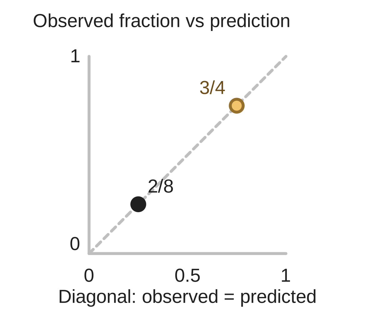
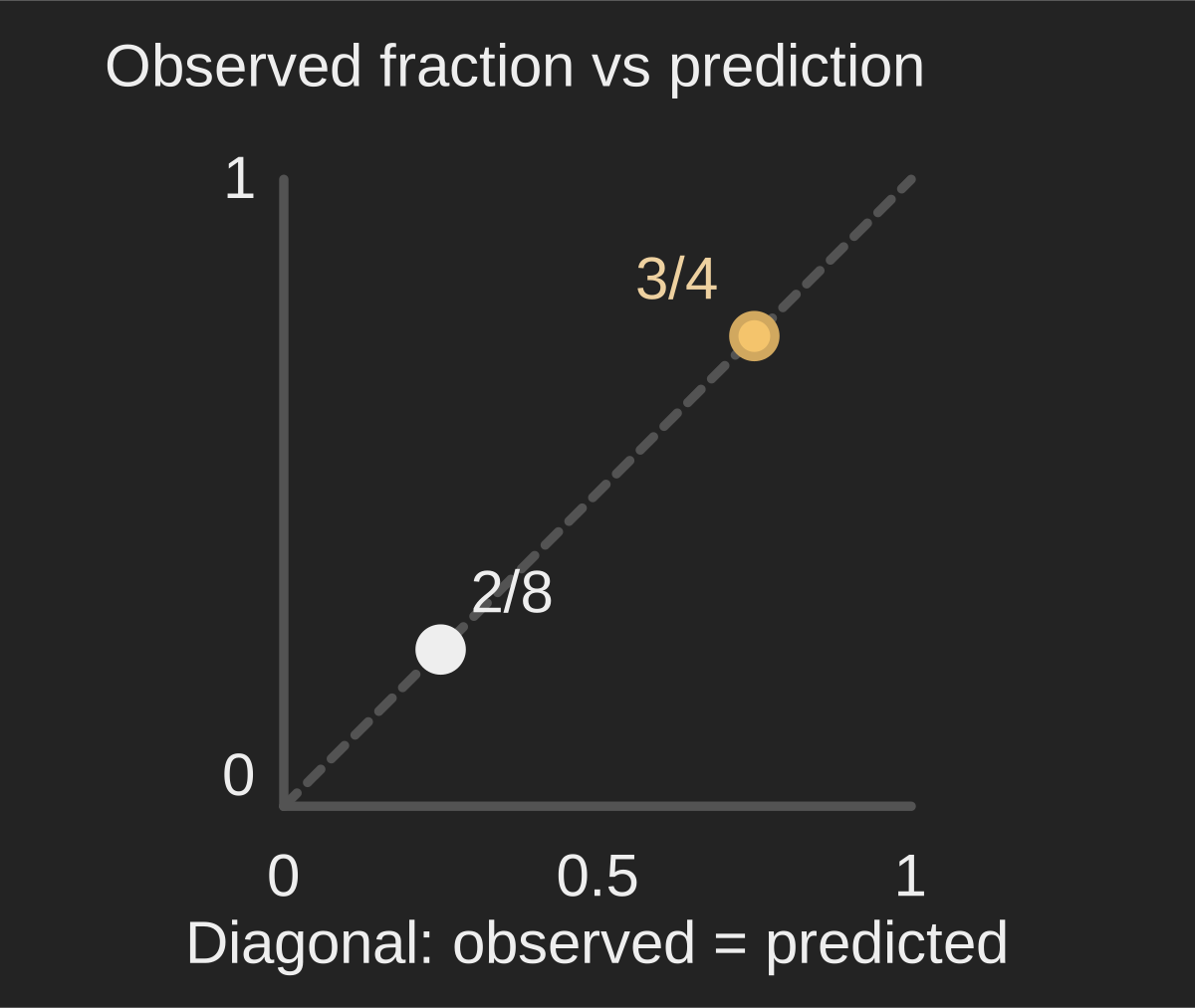
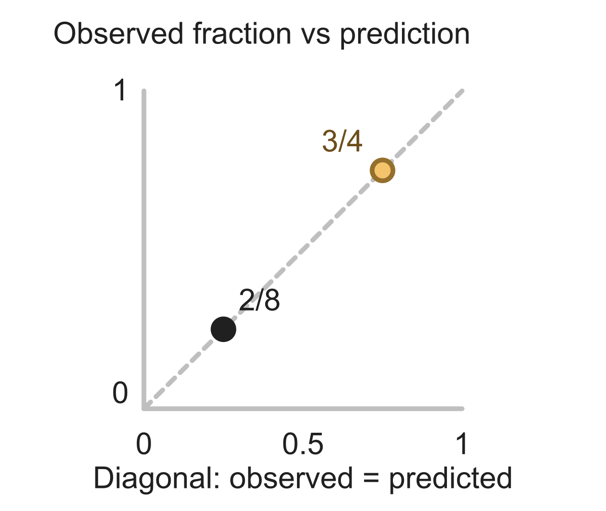
If a bin contains 20 predictions all equal to 0.7 and 10 positive labels, its mean forecast is 0.7 and observed frequency is . The absolute gap is 0.2. This one bin shows a discrepancy, but finite-sample noise means it does not establish the exact population gap.
One bin: mean prediction 0.6; 2 positives among 5. Observed fraction / comparison?
Show answer and explanation
2/5=0.4<0.6.
02Predictions within a bin can differ#
Predictions within a bin can differ. For predictions 0.1 and 0.5 with outcomes 0 and 1, average predictions to get 0.3. Average the outcomes to get 0.5. This bin’s predictions are lower than its observed frequency.
Pooling can hide errors. Two equal-size bins predict 0.1 and 0.9, but have observed fractions 0.4 and 0.6. Both pooled averages are 0.5, although neither bin matches.
One bin (prediction, 0/1 outcome): (0.2,1), (0.6,1). Mean prediction / observed fraction?
Show answer and explanation
Mean 0.4; 2/2=1.
03A closer look#
Matching a finite set of bins is empirical evidence, not proof of exact population calibration. Calibration also differs from separation: assigning everyone the same probability can match the overall frequency while giving no ranking among cases.
Bins (mean prediction; positives/total): A(.25;3/4), B(.75;1/4). “Both match by pooling.” Fractions / matches?
Show answer and explanation
0.75≠0.25 in each.
04A model can rank positive cases well while overstating their probabilities#
A model can rank positive cases well while overstating their probabilities. Conversely, a constant base-rate forecast can be calibrated while providing little discrimination. Evaluate calibration on held-out data, and consider bin counts when interpreting noisy reliability estimates.
Within every stated bin, compare the mean prediction with positives divided by the bin count. Keep empirical agreement separate from class separation or population proof.
- Compare predictions and observed frequencies within each bin.
Sources & further reading
- [1]Scikit-learn User Guide, Probability Calibration ↗Scikit-learn developers · Article