Machine learning
Gradient clipping by norm vs value: what does the limit mean?
Clip the same gradient two ways, see why their lengths differ, and check global clipping, PyTorch code, and the limits of what clipping can fix.
In this article
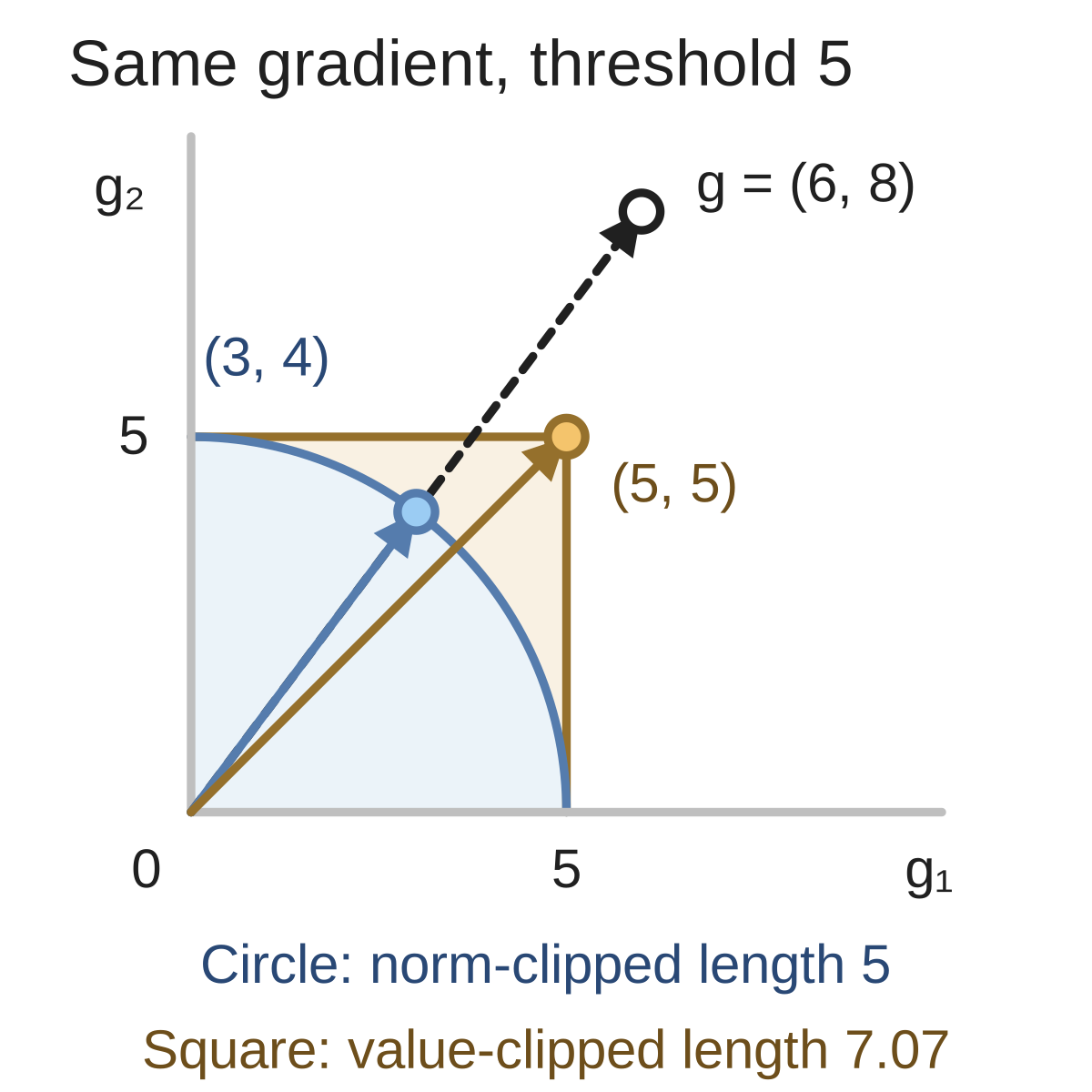
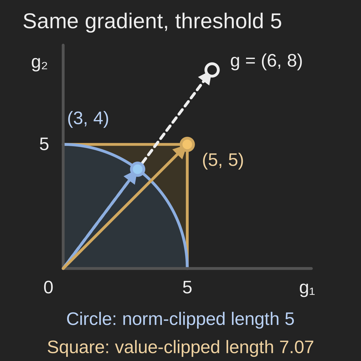
Start with the dashed gradient g = (6, 8), whose length is 10. Norm clipping reaches the blue circle at (3, 4), length 5. Value clipping reaches the amber square at (5, 5), length about 7.07. The constraints share equally scaled axes; only their first quadrants are shown.
Original illustrative calculation, not a training benchmark. Values follow the two clipping definitions.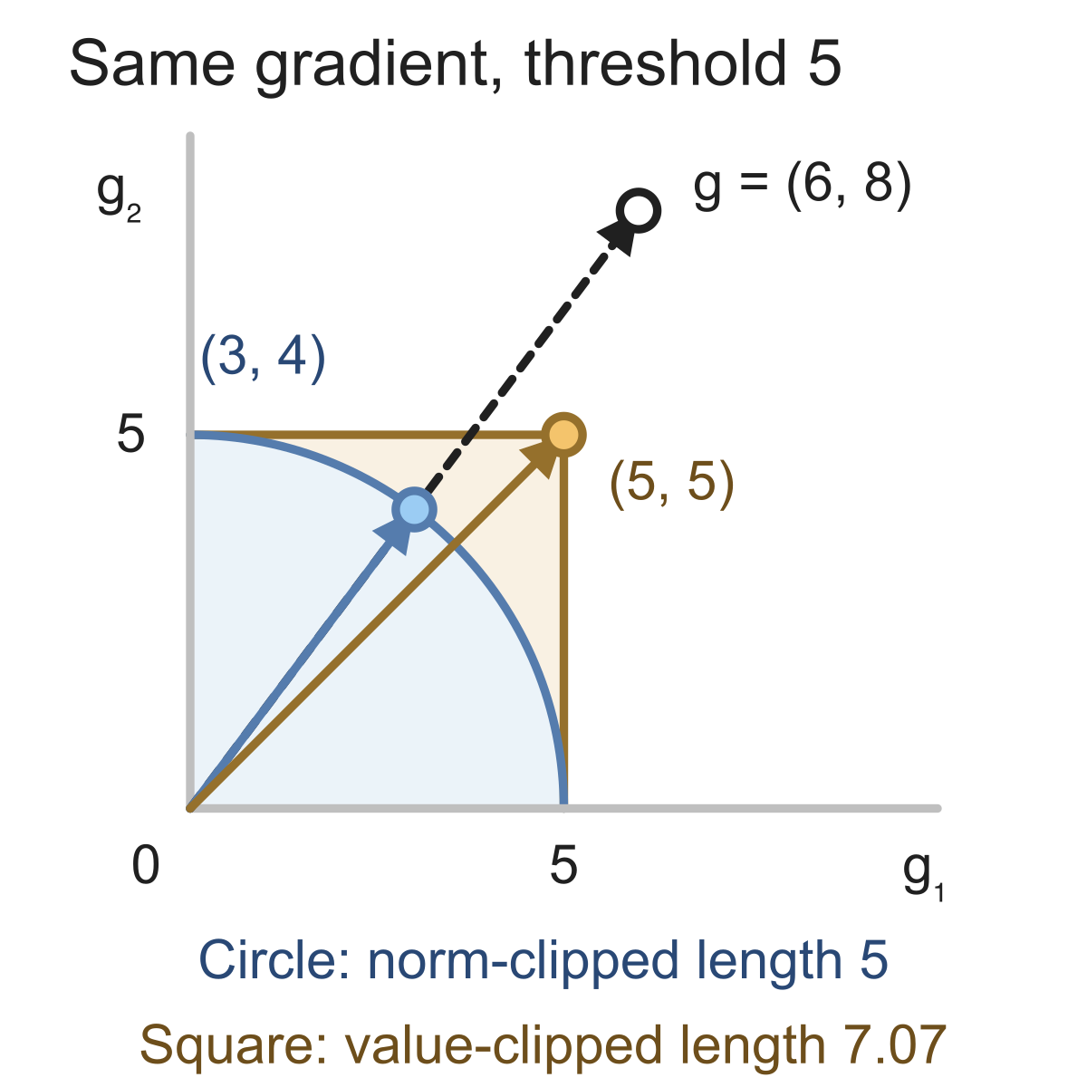
A gradient clipped at 5 can still have a length greater than 5. Take . Clipping each entry at 5 gives , whose length is about . Clipping the gradient's length at 5 gives instead.
Both operations are called gradient clipping. The first limits individual coordinates; the second limits the norm of the whole vector. That distinction matters when you choose a threshold, compare training code, or try to understand how much an update can move the parameters.
You only need vector length and the ordinary gradient-descent update to follow the example. The small vectors below are illustrative calculations, not measurements from a training run.
Where clipping belongs in a training step
Backpropagation computes a gradient . Before the optimizer uses it, clipping replaces it with a bounded version . For plain gradient descent, the update becomes
The learning rate scales the gradient on every step. Norm clipping changes the gradient only when its length exceeds the chosen cap. If the cap is rarely reached, most steps are unchanged.
Large gradients can arise when derivatives compound through a network. Pascanu and colleagues analyzed this problem in recurrent networks and proposed gradient-norm clipping to address exploding gradients. Clipping does not change the backward-pass calculation itself. It changes the gradient supplied to the optimizer, as a separate step after backward. Our backpropagation and gradient-descent example shows those stages before adding clipping.
Clip by norm: shorten the whole vector
For a positive threshold , L2-norm clipping is
The zero vector stays zero. Every coordinate of a vector above the threshold receives the same positive multiplier, so its direction is preserved.
For our gradient, . With , the multiplier is . The result is
The ratio between coordinates remains . Geometrically, the endpoint moves toward the origin along the original ray until it reaches the radius-5 circle. This is different from always normalizing a vector: a gradient with length 2 would be left alone, not enlarged to length 5.
Clip by value: constrain each coordinate
Value clipping applies a bound separately to every entry:
At , our two entries both exceed the upper limit, so becomes . Its coordinates are allowed, but its length is . Its direction also changes: the coordinate ratio is now 1.
PyTorch's value-clipping operation uses this interval constraint. In two dimensions the allowed endpoints form a square. In dimensions, each coordinate can have magnitude , so the vector's L2 norm can reach .
Value clipping does not always rotate a vector. A vector already inside the bounds is unchanged, and some symmetric vectors retain their direction after clipping. The point is that direction preservation is not guaranteed.
| With threshold 5 | By L2 norm | By value |
|---|---|---|
| What is bounded? | The whole vector's length | Each coordinate's magnitude |
| Result for | ||
| Resulting length | ||
| Direction preserved? | Yes, for nonzero vectors | Sometimes |
Using the same threshold number does not make these equivalent settings. Pick the constraint you mean before tuning its value.
Global clipping is different from clipping each layer
A model has many parameter arrays, but a global gradient norm treats their gradient entries as one long vector. PyTorch's norm-clipping function applies one multiplier across the supplied parameters.
Suppose two parameter blocks have gradients and . Their separate lengths are 5 and 12; the global length is
With a global cap of 6.5, both blocks are halved. Block A becomes even though its own length was below the cap. The large gradient in B makes the combined gradient too long.
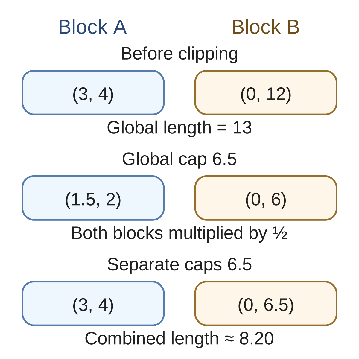
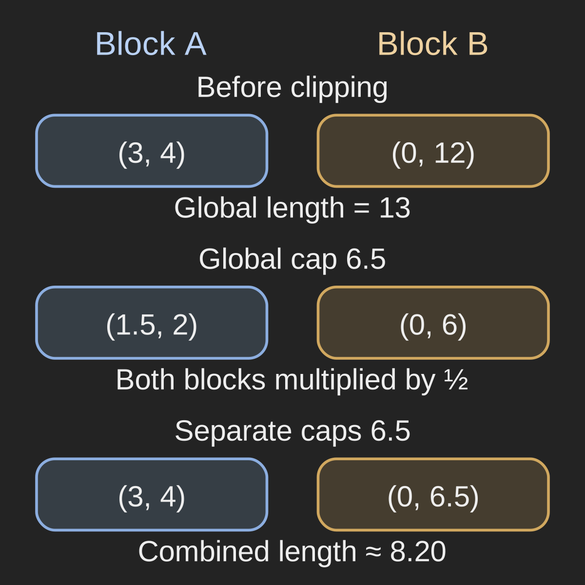
Global clipping treats both blocks as one gradient (3, 4, 0, 12), with norm 13. A cap of 6.5 halves every entry. Applying a separate cap to each block is a different operation and does not enforce a global cap of 6.5.
Original four-coordinate example; Euclidean norms calculated from the displayed entries.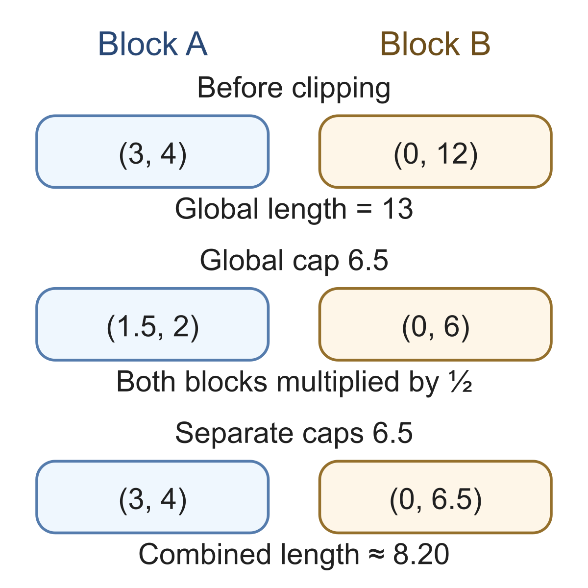
If we instead clipped each block independently at 6.5, A would remain and B would become . The combined length would be . A separate cap per layer therefore does not enforce that cap across the model.
Reproduce the numbers in Python
This example needs only Python's standard library. It deliberately checks finite inputs and a positive cap; silently carrying a NaN into an optimizer would obscure the issue we are trying to diagnose.
from math import hypot, isfinite

def clip_by_norm(values, cap):
    if not isfinite(cap) or cap <= 0:
        raise ValueError("cap must be positive and finite")
    if not all(isfinite(v) for v in values):
        raise ValueError("gradient must be finite")
    length = hypot(*values)
    scale = cap / length if length > cap else 1.0
    return tuple(scale * v for v in values)

def clip_by_value(values, cap):
    if not isfinite(cap) or cap <= 0:
        raise ValueError("cap must be positive and finite")
    if not all(isfinite(v) for v in values):
        raise ValueError("gradient must be finite")
    return tuple(max(-cap, min(cap, v)) for v in values)

g = (6.0, 8.0)
for name, result in [
    ("norm", clip_by_norm(g, 5.0)),
    ("value", clip_by_value(g, 5.0)),
]:
    print(name, result, round(hypot(*result), 6))

global_result = clip_by_norm((3.0, 4.0, 0.0, 12.0), 6.5)
print("global", global_result, hypot(*global_result))
norm (3.0, 4.0) 5.0
value (5.0, 5.0) 7.071068
global (1.5, 2.0, 0.0, 6.0) 6.5
Here is a complete PyTorch example using a linear loss solely to produce the same gradient. The underscore in the clipping function's name indicates that it modifies the stored gradients in place. Its return value is the total norm before clipping.
import torch

theta = torch.nn.Parameter(torch.zeros(2, dtype=torch.float64))
optimizer = torch.optim.SGD([theta], lr=0.1)

optimizer.zero_grad(set_to_none=True)
loss = (theta * torch.tensor([6.0, 8.0])).sum()
loss.backward()

before = torch.nn.utils.clip_grad_norm_(
    [theta], max_norm=5.0, error_if_nonfinite=True
)
print("before:", round(before.item(), 6))
print("gradient:", [round(v, 6) for v in theta.grad.tolist()])
optimizer.step()
print("parameters:", [round(v, 6) for v in theta.tolist()])
The output is a pre-clipping norm of 10, a gradient approximately , and updated parameters approximately . Small numerical differences are expected because the implementation uses floating-point arithmetic and a stabilizing term. This linear loss is a gradient demonstration, not a model-training recipe.
With mixed precision, clipping must operate on the unscaled gradients. Complete accumulation for the optimizer step, call scaler.unscale_(optimizer), clip, and then call scaler.step(optimizer) and scaler.update(). The PyTorch mixed-precision examples explain the ordering. Clipping each microbatch separately generally differs from clipping the final accumulated gradient because clipping is nonlinear.
What a clipping threshold cannot promise
For plain gradient descent without momentum or weight decay, L2-norm clipping gives a useful bound:
A bounded step can still be too large. Consider , starting at , with learning rate 3 and cap 1. The first gradient, 0.5, is already below the cap. The update reaches , increasing the loss from 0.125 to 0.5. The next steps alternate between and . Every clipped gradient obeys the cap; the method still fails to converge. The oscillating-gradient-descent article explains why step size matters on this quadratic.
The same bound does not generally apply to the full update of momentum or Adam. Those optimizers also use stored state, and Adam rescales coordinates using second-moment estimates. The optimizer equations in Google's tuning playbook make the extra operations explicit.
Choose a threshold by inspecting the unclipped gradient norms and checking the resulting training behavior. Google's playbook recommends recording the norms over time and looking at their distribution; its suggested thresholds are starting points for a workload, not universal constants. If clipping activates almost every step, investigate whether the learning rate or loss scaling needs attention. If gradients are already nonfinite, investigate that numerical failure rather than expecting clipping to repair it.
Once the gradient is finite and the intended bound is clear, the implementation question becomes precise: which parameter gradients belong in the same vector, and at what point in the update should that vector be limited?
Learn with Glacius
Want to go deeper into the math?
Build your understanding with visual lessons and practice on the concepts from this article.
Check the reasoning
Sources & notes
- PyTorch: clip_grad_norm_ ↗
Global norm, in-place modification, and the returned norm.
- PyTorch: clip_grad_value_ ↗
Coordinate-wise clipping to a symmetric interval.
- PyTorch: automatic mixed precision examples ↗
Unscale after accumulating gradients and before clipping.
- Google Deep Learning Tuning Playbook: optimization failures ↗
Monitoring unclipped gradient norms, selecting a threshold, and optimizer update equations.
- Pascanu, Mikolov and Bengio: On the difficulty of training Recurrent Neural Networks ↗
Analysis of exploding and vanishing gradients and a gradient-norm clipping strategy.
Our figures use illustrative mathematical examples unless a dataset is explicitly identified. You can share the original Glacius figures with attribution and a link to this article; linked third-party material retains its own terms.
Keep exploring