Machine learning
Normalization vs standardization: what happens to an outlier?
Compare min–max scaling and z-scores on one small column. See why skew survives, how outliers change both methods, and why test values can exceed 1.
In this article
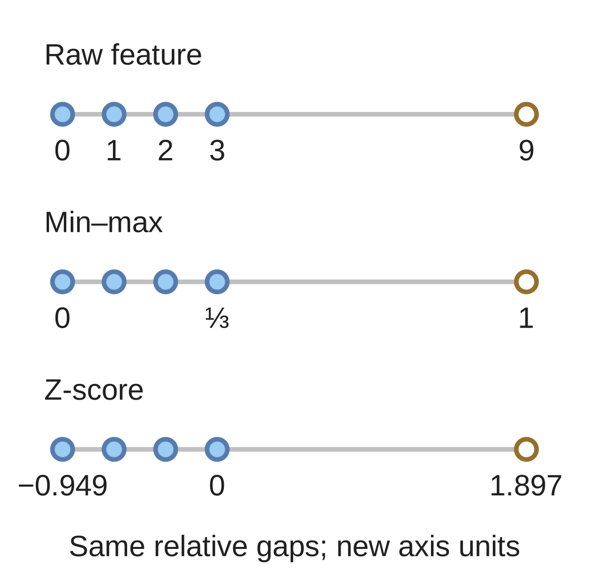
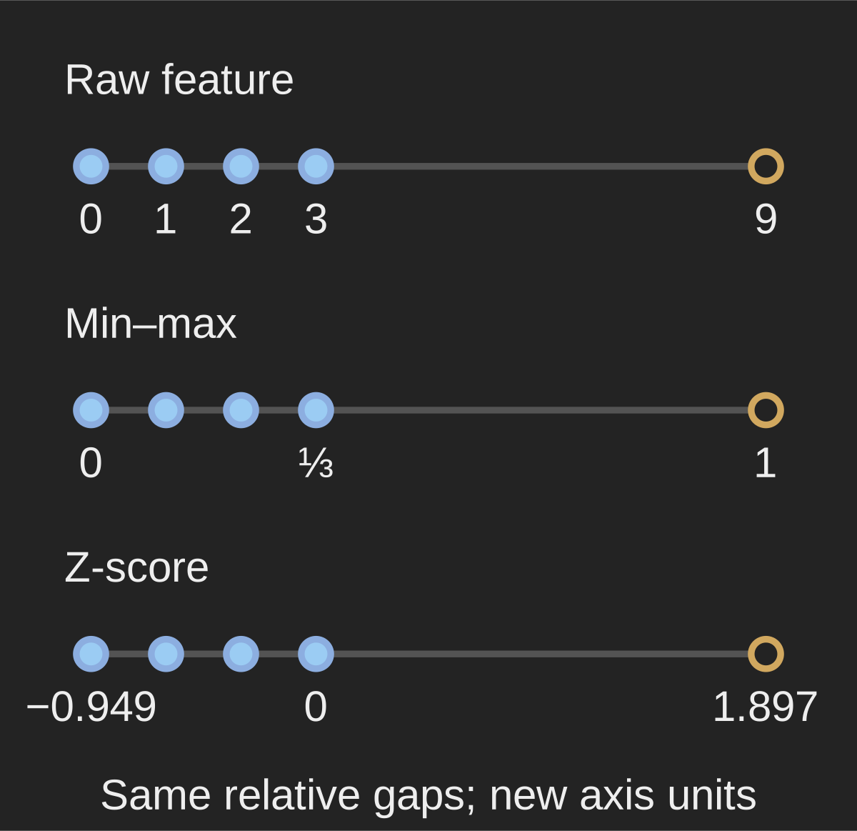
Each row spans its own minimum and maximum. The five observations occupy identical relative positions because both transformations shift and stretch a single axis. The large final gap survives. Hollow amber markers identify the largest observation; z-scores are rounded to three decimals.
Original illustrative column [0, 1, 2, 3, 9], calculated by Glacius. Population mean 3 and standard deviation √10; no measured dataset.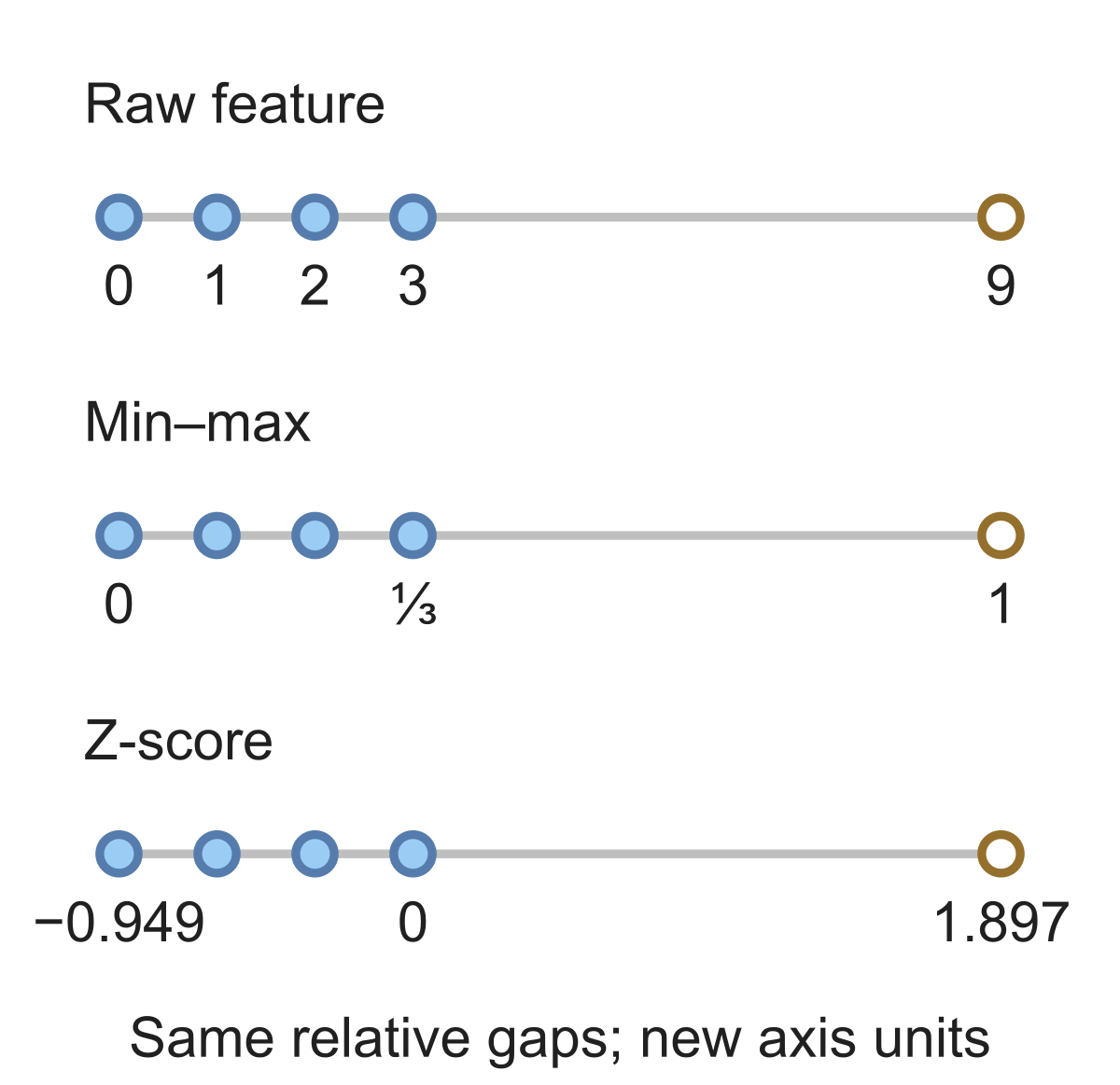
One added value can squeeze four training observations from the entire 0–1 interval into its first third. Start with the illustrative column , apply min–max scaling, then add and fit again. The original values now occupy because the fitted range has tripled.
Would standardization fix that? It changes which quantities set the scale, but the added value still affects every result. Understanding that effect is more useful than memorizing which algorithms supposedly want which scaler.
Min–max normalization subtracts a feature's training minimum and divides by its training range. Standardization subtracts its training mean and divides by its training standard deviation. Both operate on each feature column separately. Neither removes outliers or turns a skewed distribution into a bell curve.
The word normalization has several meanings. Here it means min–max feature scaling. In our cosine similarity and Euclidean distance article, normalization means dividing an individual vector by its length. That acts across a row of coordinates, rather than down a column of observations. Scikit-learn's Normalizer implements that separate operation.
Two formulas, one training column
Keep the added value and use this five-row training column throughout:
These are chosen numbers, without physical units or a measured population behind them. Four values are close together; the fifth sits well to their right.
For the usual 0–1 output range, the min–max transformation is
Here and , so we divide each observation by nine. In particular, becomes and becomes . The endpoints describe the data used to fit the scaler; they are not a promise about every future input. That training-set qualification is part of the MinMaxScaler definition.
Standardization instead uses
Our training mean is . To calculate the standard deviation, square each distance from that mean, average the squares, and take a square root:
The denominator is , rather than , matching StandardScaler's ddof=0 convention. Our standard deviation lesson develops what this measure of spread tells you.
| Original value | Min–max value | Z-score |
|---|---|---|
| 0 | 0 | −0.949 |
| 1 | 0.111 | −0.632 |
| 2 | 0.222 | −0.316 |
| 3 | 0.333 | 0 |
| 9 | 1 | 1.897 |
Values in the table are rounded to three decimals. Before rounding, the z-scores have mean zero and variance one. A z-score of zero means “at the fitted training mean”; it says nothing about the original minimum. A value of is about fitted standard deviations above that mean.
Standardization does not make data normally distributed
In the original column, adjacent gaps are . After min–max scaling they are . After standardization they are . The last gap is six times each small gap under every representation.
This follows directly from the formulas. Once fitted, either transformation has the form with for a nonconstant feature. Subtraction moves the whole column, and multiplication stretches or shrinks it uniformly. They cannot bend its long tail into a different shape. Standardization does not require Gaussian data to be mathematically defined, and zero mean with unit variance does not imply a normal distribution.
The figure above deliberately lets each axis span its own transformed minimum and maximum. That makes the preserved shape visible; it does not claim the three axes share numeric units. If a genuinely Gaussian variable is standardized with its population parameters, it becomes standard normal. Our five-point example remains a five-point example.
Both methods respond to an outlier
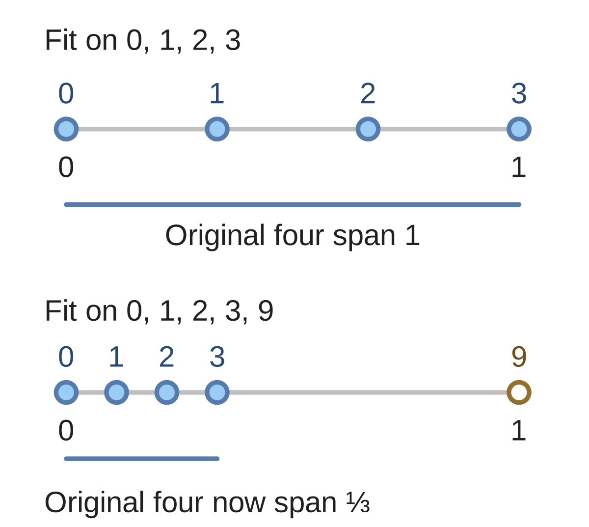
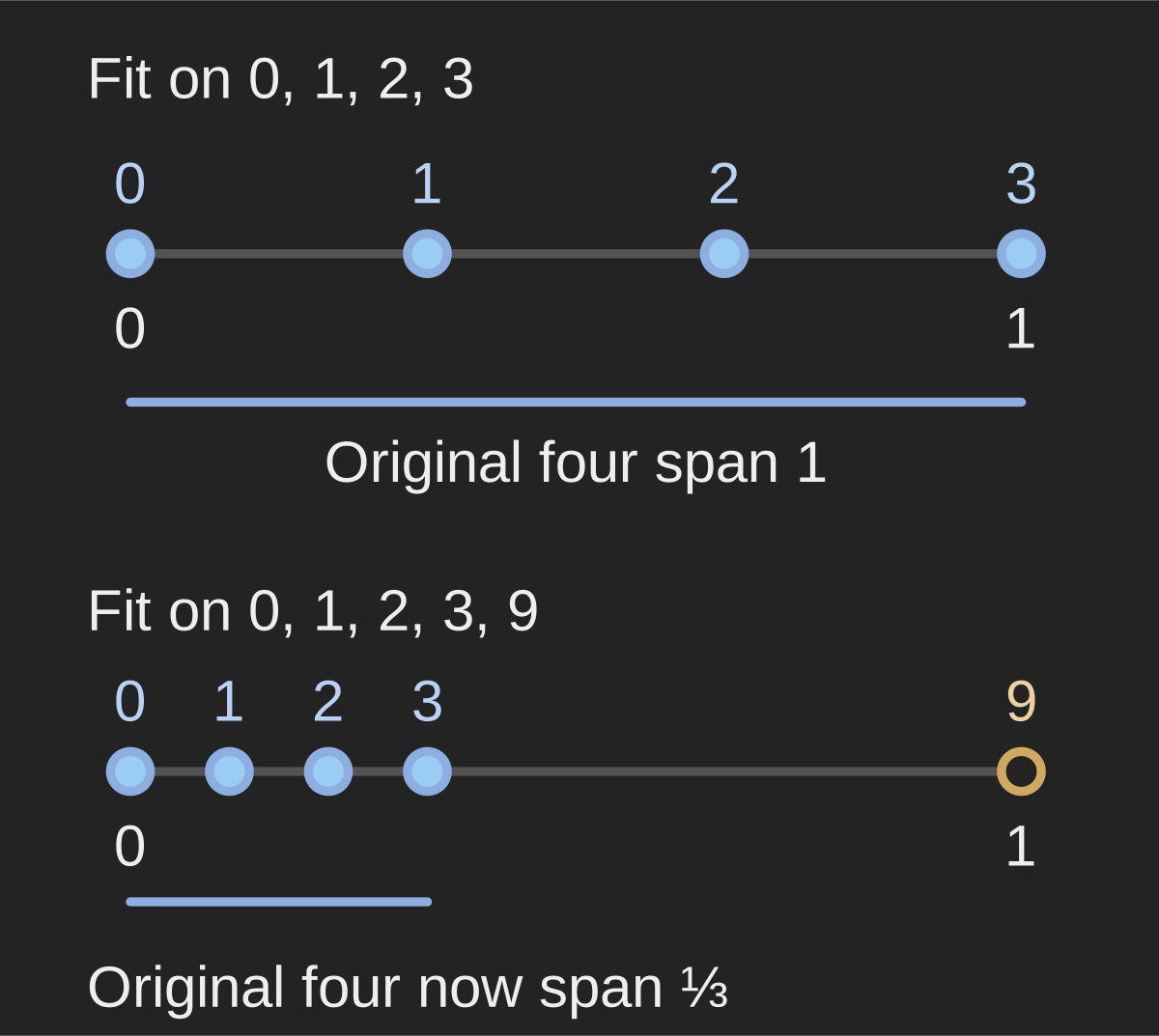
Both rows use the same 0–1 output scale. Numbers above the markers identify the original observations. Adding 9 to the training column changes the denominator from 3 to 9, so the original four values occupy only the first third of the interval.
Original controlled calculation by Glacius, comparing fits on [0, 1, 2, 3] and [0, 1, 2, 3, 9]. This is an illustrative example, not a reported dataset statistic.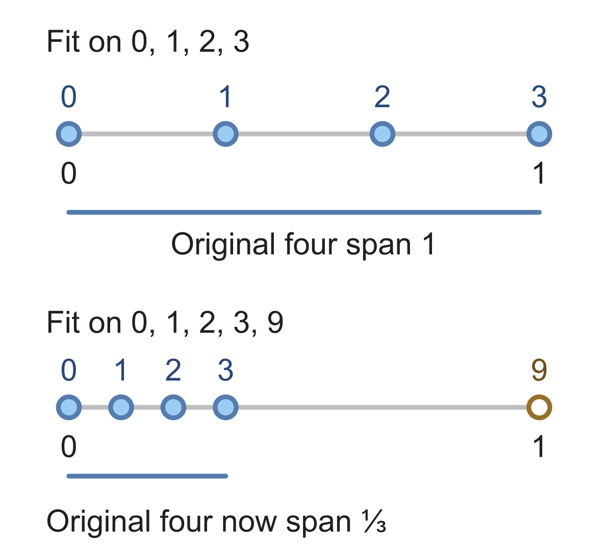
Before we added , min–max scaling divided by . Afterward, it divides by . The original four values still have distinct, correctly ordered outputs, but their span shrinks from to . Scaling has not decided whether the new observation is a valid extreme, a sensor fault, or a typing error.
Standardization also changes when we add it. For , the mean is and the standard deviation is . Adding moves the mean to and raises the standard deviation to .
The original four observations span about z-score units before the addition, but only afterward. Every value has moved because both the center and the scale changed. The value is just standard deviations above the new mean, which also shows why an extreme observation need not produce an enormous z-score when it helped determine the mean and standard deviation.
These calculations illustrate the scikit-learn comparison of scalers with outliers: both methods can compress most observations when extremes influence the fit. The two output intervals have different meanings, so a wider numeric interval alone does not prove that one method handled the outlier better.
Fit on training data; reuse the fit on test data
Suppose the next observation is . With the fitted training minimum of and maximum of , its min–max value is
An output above one is expected here. For a nonconstant feature, any input above the fitted training maximum maps above one; an input below the fitted minimum maps below zero. Refitting on the test set to keep its values in range would give it a different coordinate system and let held-out information influence preprocessing.
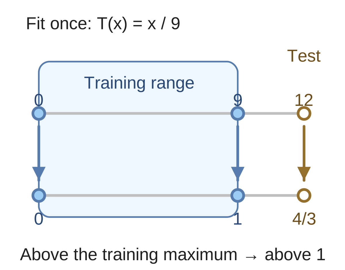
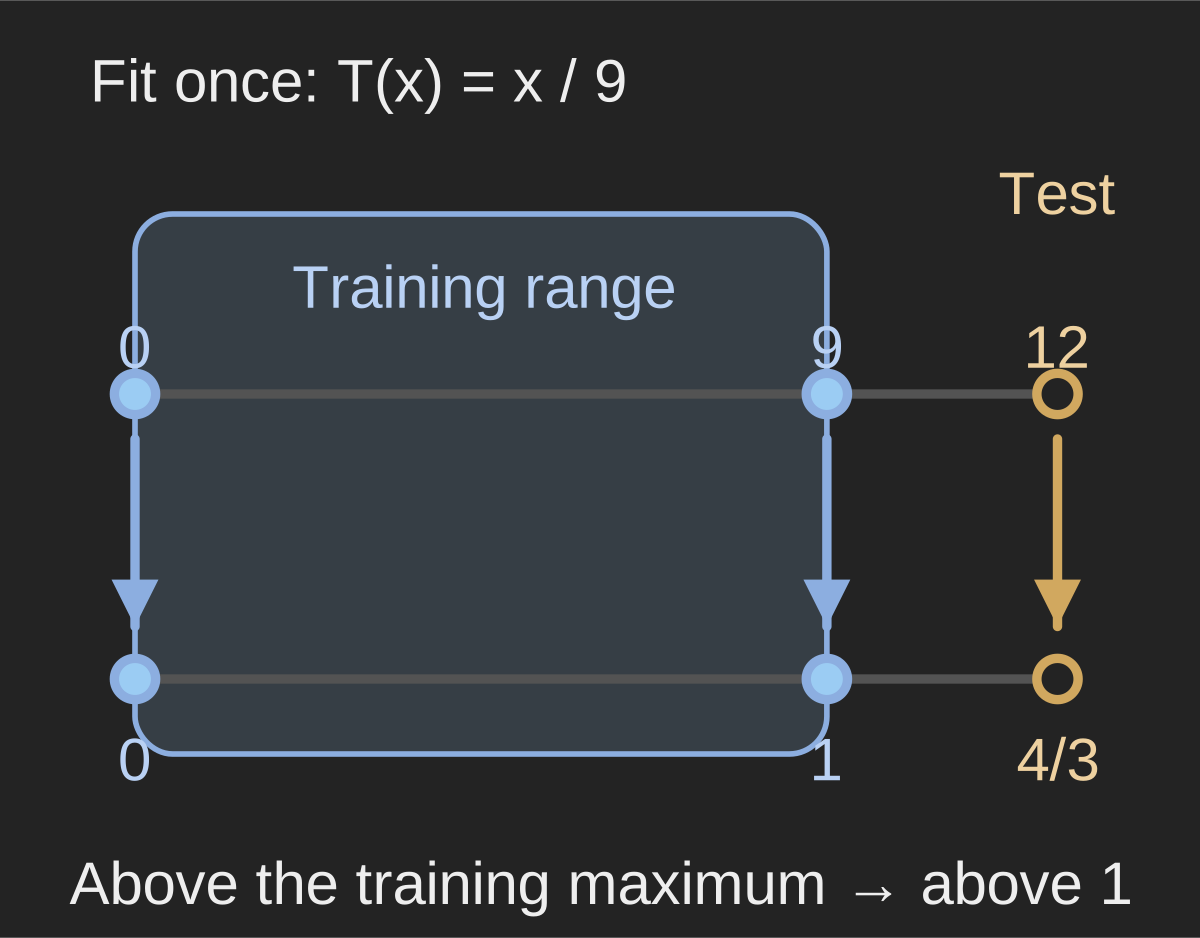
The fitted training minimum is 0 and maximum is 9. Reusing those values sends a held-out observation of 12 to 12/9 = 4/3. The shaded range belongs to the training fit; it is not a bound on future observations. Clipping is off.
Original calculation by Glacius using the documented MinMaxScaler transformation, with default clip=False.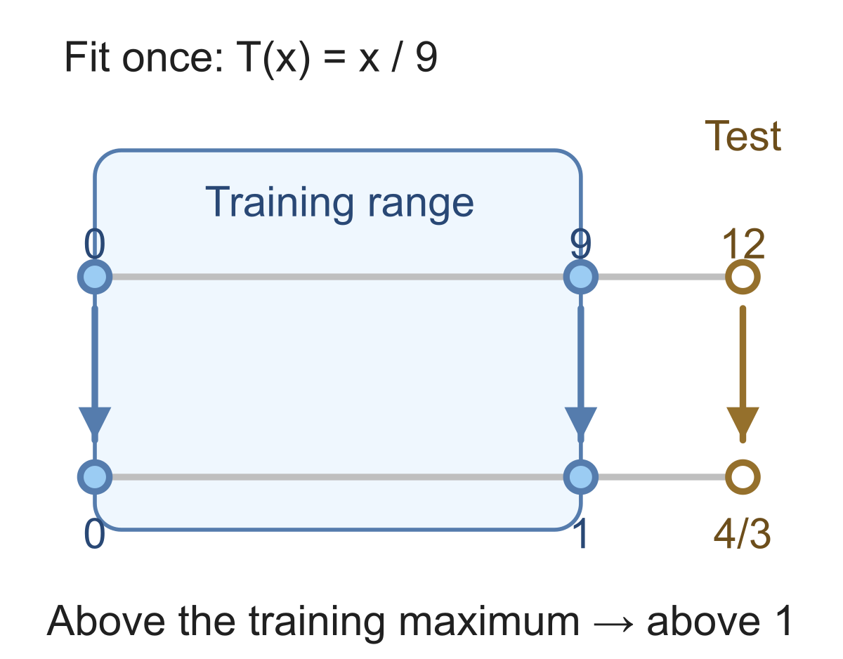
The same rule applies to standardization. We reuse and , giving . The test data need not have mean zero or standard deviation one. Those are properties of the nonconstant column used for fitting, with centering and scaling enabled.
Scikit-learn's guidance on avoiding data leakage recommends splitting first, fitting preprocessing on training data only, and transforming held-out data with that fitted object. During cross-validation, put the scaler and estimator in one pipeline so that each fold fits its own training statistics.
Check the numbers in Python
This code uses scikit-learn's defaults: population variance for StandardScaler, and no clipping for MinMaxScaler. Each row contains one sample with one feature.
import numpy as np
from sklearn.preprocessing import MinMaxScaler, StandardScaler

X_train = np.array([0., 1., 2., 3., 9.]).reshape(-1, 1)
X_test = np.array([12.]).reshape(-1, 1)

minmax = MinMaxScaler().fit(X_train)
standard = StandardScaler().fit(X_train)

mm_train = minmax.transform(X_train)
z_train = standard.transform(X_train)

print("min-max:", mm_train.ravel().round(3))
print("z-scores:", z_train.ravel().round(3))
print("test min-max:", minmax.transform(X_test).ravel().round(3))
print("test z-score:", standard.transform(X_test).ravel().round(3))

np.testing.assert_allclose(mm_train, X_train / 9)
np.testing.assert_allclose(z_train, (X_train - 3) / np.sqrt(10))
np.testing.assert_allclose(z_train.mean(axis=0), 0, atol=1e-12)
np.testing.assert_allclose(z_train.var(axis=0, ddof=0), 1)
The output is:
min-max: [0.    0.111 0.222 0.333 1.   ]
z-scores: [-0.949 -0.632 -0.316  0.     1.897]
test min-max: [1.333]
test z-score: [2.846]
Using MinMaxScaler(clip=True) would force the transformed test value down to . That is an additional clipping decision, not a different estimate of the range. It makes and every larger input beyond the maximum share the same output, so information is lost. The API documentation warns that clipping can distort held-out data and prevent exact inversion.
Choose the scale that matches the model
In a distance-based model, changing feature scales changes how much each feature contributes. For example, after per-feature standardization, the squared distance between two rows contains terms of the form . A feature with twice the fitted standard deviation contributes one quarter as much for the same raw difference. This is a modeling choice about relative differences, not a guarantee that every feature becomes equally useful.
Min–max scaling is useful when the fitted range is the reference you want. When bounds are known from the measurement itself, such as an 8-bit pixel's range of 0 to 255, dividing by the known upper bound is a separate, fixed choice; you need not estimate that bound from a batch. If later inputs must stay inside a strict interval, decide explicitly how invalid or out-of-range values should be handled.
Standardization is useful when deviations from a fitted center provide a sensible common scale. It is a candidate for models sensitive to feature magnitudes, including many distance-based or regularized models. Neither method wins for every dataset. Compare suitable alternatives using training folds and validation results, while keeping the final test set separate. Decision trees based on feature thresholds generally do not need this kind of scaling, as the scikit-learn scaling comparison explains.
If extremes dominate your fit, inspect what they represent before choosing a remedy. A median-and-interquartile-range scaler can reduce their influence on the fitted scale. A nonlinear transformation addresses a different question: whether to change distribution shape. Neither operation establishes that the observations themselves are wrong.
What if a column never changes?
For a constant training column such as , the range and standard deviation are both zero. The two raw formulas would divide by zero. No affine transformation can turn a constant column into one with unit variance.
With its default centering enabled, scikit-learn's StandardScaler uses a scale factor of one in this case, so the training values become zero. MinMaxScaler with its default range also maps a constant training column to zero through its zero-range handling. Those outputs are software conventions for a degenerate feature, not evidence that it acquired useful variation. Decide how to handle such columns in the training pipeline, and pay attention if a supposedly constant feature starts varying after deployment.
For the column we worked through, both denominators are nonzero and the transformations are reversible before clipping and rounding. You can recover an original value from a z-score using . Try that with and with ; our standardization lesson develops this forward-and-backward interpretation.
Learn with Glacius
Want to go deeper into the math?
Build your understanding with visual lessons and practice on the concepts from this article.
Check the reasoning
Sources & notes
- scikit-learn: StandardScaler ↗
Per-feature centering and scaling, sensitivity to outliers, ddof=0, and zero-variance handling.
- scikit-learn: MinMaxScaler ↗
Training-range scaling, default clip=False, and the limits of clipping held-out observations.
- scikit-learn: Compare the effect of different scalers on data with outliers ↗
Both standard scaling and min–max scaling are sensitive to outliers; robust and nonlinear transformations solve different problems.
- scikit-learn: Common pitfalls and recommended practices ↗
Fit preprocessing on training data only, reuse transform on held-out data, and use pipelines during cross-validation.
- scikit-learn: Normalizer ↗
Unit-norm scaling acts on individual sample vectors, a different operation from scaling feature columns.
Our figures use illustrative mathematical examples unless a dataset is explicitly identified. You can share the original Glacius figures with attribution and a link to this article; linked third-party material retains its own terms.
Keep exploring