Machine learning
Ridge vs lasso: why one coefficient becomes zero
Follow the same two coefficients through ridge and lasso, derive the zero threshold, and see why correlated features complicate feature selection.
In this article
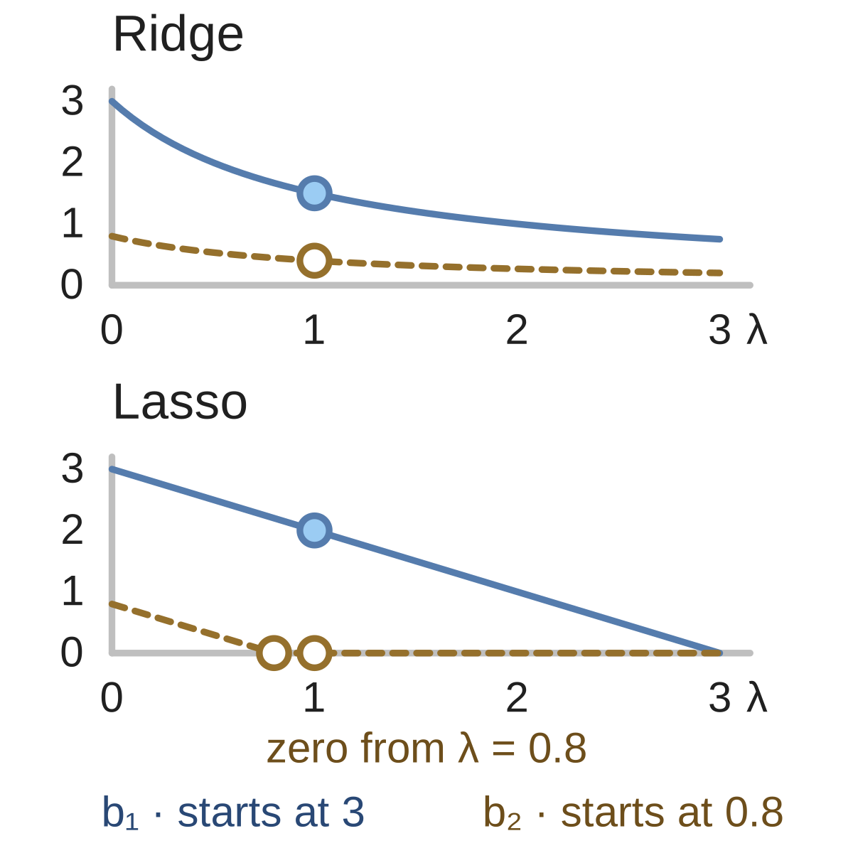
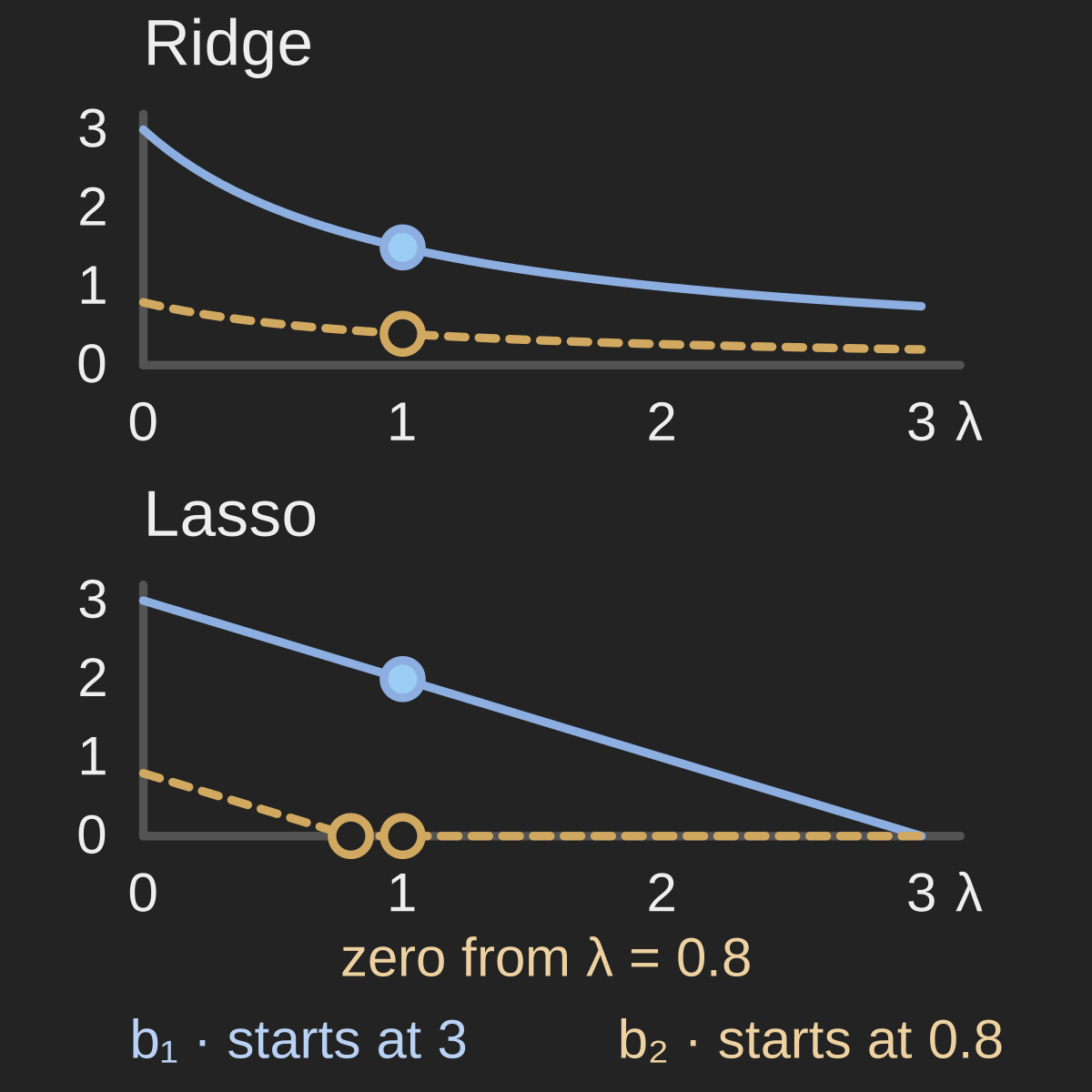
Original four-row example with orthogonal, centered features of mean square one. Solid blue is b₁, initially 3; dashed amber is b₂, initially 0.8. Both panels use the same coefficient and λ scales. Markers show λ = 1. These formulas apply to this orthogonal design, not every regression dataset.
Calculated from ridge b = z/(1+λ) and lasso b = sign(z) max(|z|−λ, 0), with the objective conventions stated in the article.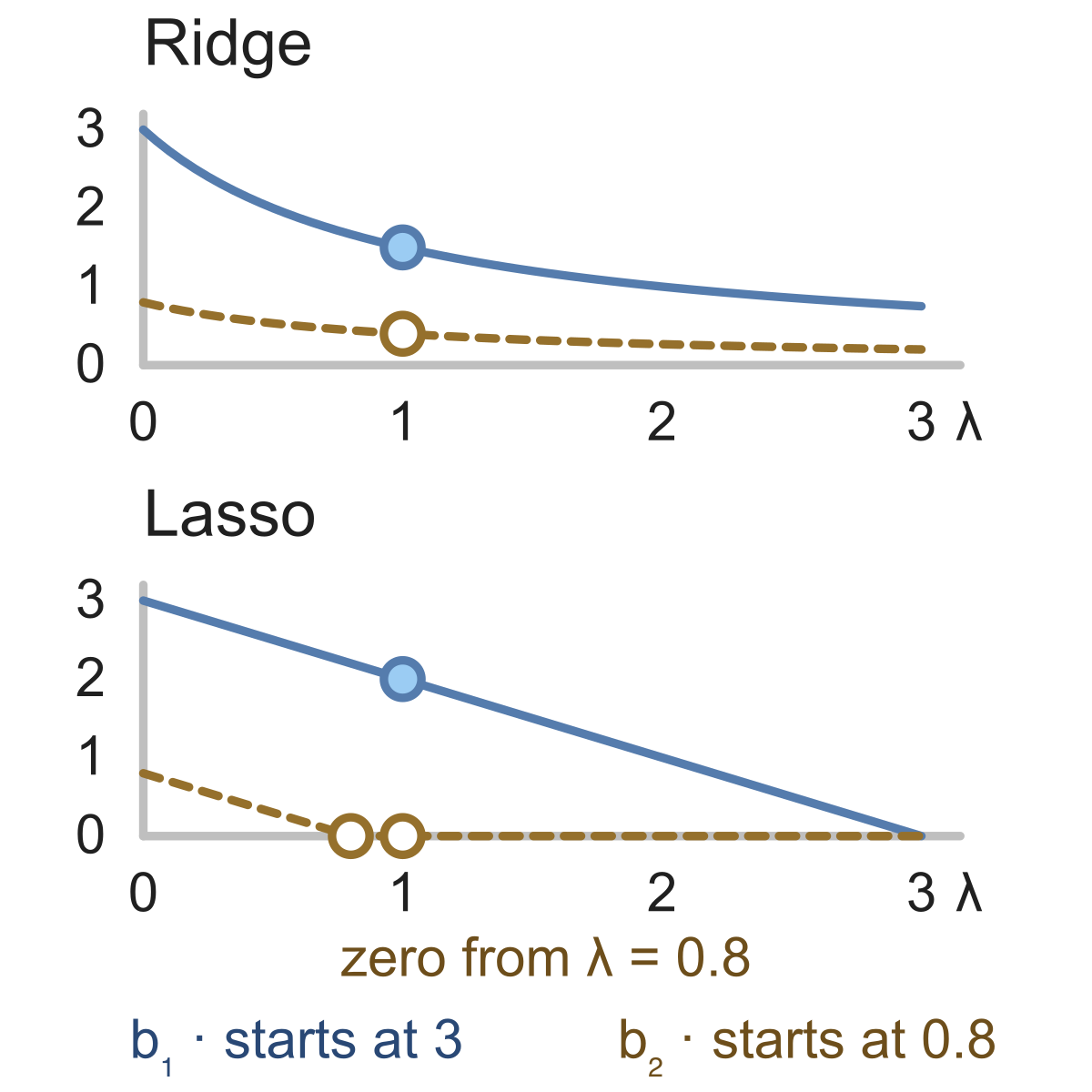
A fitted linear model has two coefficients: and . Add a ridge penalty and, in the example below, they become and . Add a lasso penalty and they become and . Both fits accept more training error in exchange for smaller coefficients. Only the second has removed a feature from its prediction.
The difference comes from the penalty near zero. Ridge penalizes squared coefficients, so its pull toward zero weakens as a coefficient gets smaller. Lasso penalizes absolute values and can make zero the exact optimum over a whole range of inputs. That is the basis of lasso's feature selection, although a selected feature is not necessarily the uniquely important one.
We can derive those four numbers from a dataset small enough to inspect, then change the dataset to see where the feature-selection interpretation breaks down. You will need linear regression and basic derivatives; the matrix notation only packages the four rows.
Give both methods the same data
Our synthetic dataset has four observations and two features. The prediction is .
| Observation | |||
|---|---|---|---|
| A | 1 | 1 | 3.8 |
| B | 1 | −1 | 2.2 |
| C | −1 | 1 | −2.2 |
| D | −1 | −1 | −3.8 |
These values were constructed as . There is no noise, and ordinary least squares recovers with zero training error. This is a calculation about penalties, not evidence about predictive performance on new data.
Both feature columns have mean zero and mean square one. Their dot product is zero: knowing one column does not help reconstruct the other through a linear combination. If is the matrix of feature values and , those properties give . The response is also centered, so the fitted intercept is zero; we leave it out of the calculation.
Use the following objective conventions throughout:
Here controls the penalty. The factor of in the ridge penalty simplifies its derivative. These are standard forms, but libraries differ in how they scale the loss and name the penalty parameter. We will translate them into scikit-learn's alpha below.
Because our columns are orthogonal and scaled, the data-loss term simplifies to
Each coefficient can now be optimized separately. This separation is a convenience of the example; it does not hold for arbitrary correlated features.
Ridge divides; lasso subtracts until it reaches zero
Write for one unpenalized coefficient, either or . Its ridge objective is
Setting the derivative to zero gives , so
At , ridge halves both coefficients: . For either nonzero in this example, any finite penalty leaves a nonzero result. If were already zero, ridge would return zero too. “Ridge never produces a zero coefficient” is therefore too strong; it has no lasso-like interval that thresholds small nonzero values to zero.
Lasso replaces the squared penalty with . On the positive side, its derivative is , which suggests . That solution works only while it stays positive. On the negative side, the derivative is , giving while that value is negative.
At zero, look at the slopes from each side. The slope just to the left is ; just to the right it is . Zero minimizes this convex objective when the left slope is nonpositive and the right slope is nonnegative, which happens exactly when . Combining the cases gives soft thresholding:
At , the coefficient becomes , while becomes zero. Lasso is solving a different optimization problem, rather than rounding a small ridge coefficient after fitting.
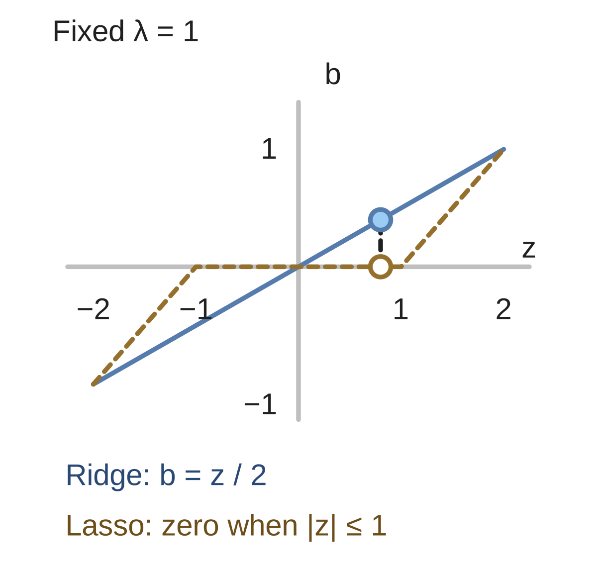
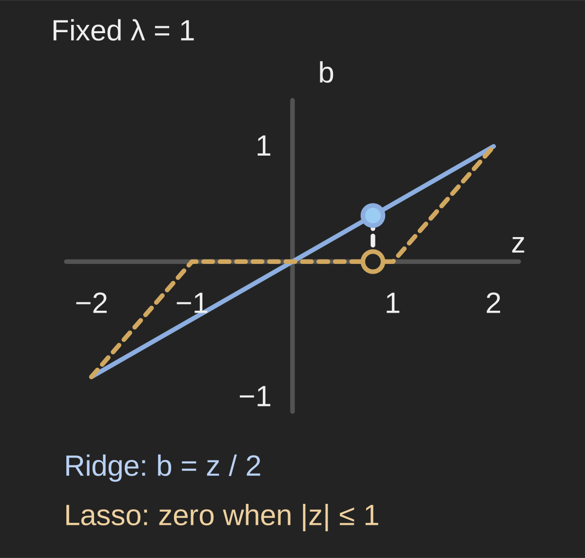
Hold λ = 1 and vary an unpenalized coefficient z in the orthogonal example. The solid ridge line crosses zero only at z = 0. The dashed lasso line stays at zero from −1 to 1. The paired markers show z = 0.8: ridge gives 0.4 and lasso gives zero.
Exact one-coordinate solutions to the objectives in the article; an illustrative calculation, not measured data.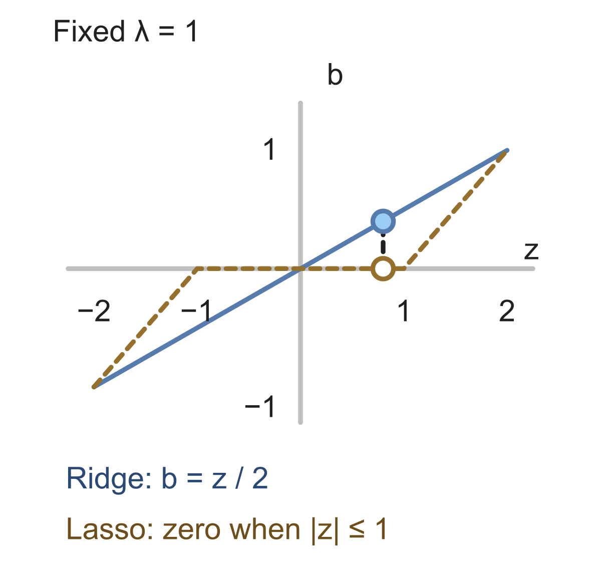
The regularization paths in the opening figure follow these formulas as increases. Ridge's coefficients approach zero smoothly. Lasso's smaller coefficient reaches zero at , and its larger coefficient reaches zero at . These simple monotone paths depend on our orthogonal design; individual paths with correlated predictors can behave differently.
Reproduce the coefficients in Python
The scikit-learn Ridge objective is the sum of squared residuals plus alpha times the squared coefficient norm. Multiply our ridge objective by and you get that form with alpha = n * lambda.
The scikit-learn Lasso objective already divides the squared residuals by , so its alpha equals our . Using the same numerical alpha in both estimators would not reproduce the conventions above. Even after this conversion, a shared is an illustrative setting, not a claim that both models have equally strong regularization or equally good validation performance.
import numpy as np
from sklearn.linear_model import Ridge, Lasso

X = np.array([[1, 1], [1, -1], [-1, 1], [-1, -1]], dtype=float)
y = X @ np.array([3.0, 0.8])
n = len(y)
lam = 1.0

# X and y are already centered; feature mean squares are one.
ridge = Ridge(alpha=n * lam, fit_intercept=False, solver="svd")
lasso = Lasso(alpha=lam, fit_intercept=False, tol=1e-12,
              max_iter=10000)

for name, model in [("ridge", ridge), ("lasso", lasso)]:
    model.fit(X, y)
    mse = np.mean((y - model.predict(X)) ** 2)
    print(f"{name}: coefficients={model.coef_.round(4)}, mse={mse:.4f}")
The output is:
ridge: coefficients=[1.5 0.4], mse=2.4100
lasso: coefficients=[2. 0.], mse=1.6400
Neither training error beats the unpenalized fit, which is exact. Lasso's lower training error at this particular setting does not establish that lasso is the better predictor. Regularization deliberately changes the training objective; its value on unseen data must be checked separately.
A zero coefficient does not settle which feature matters
Now replace the two different columns with two copies of the same centered, unit-variance feature , and let . A prediction uses only the sum of the coefficients:
At , the lasso objective becomes
Fix a nonnegative total . Every nonnegative split of that total has the same penalty, . Minimizing gives . Thus , , and all minimize the same lasso objective and produce identical predictions. A solver can return a sparse answer, but the data have not established that one of the duplicate features deserves the credit.
For ridge, a fixed total has the smallest squared penalty when the coefficients share it equally: . Substitution gives , whose minimum is also at this setting. Ridge has the unique solution .
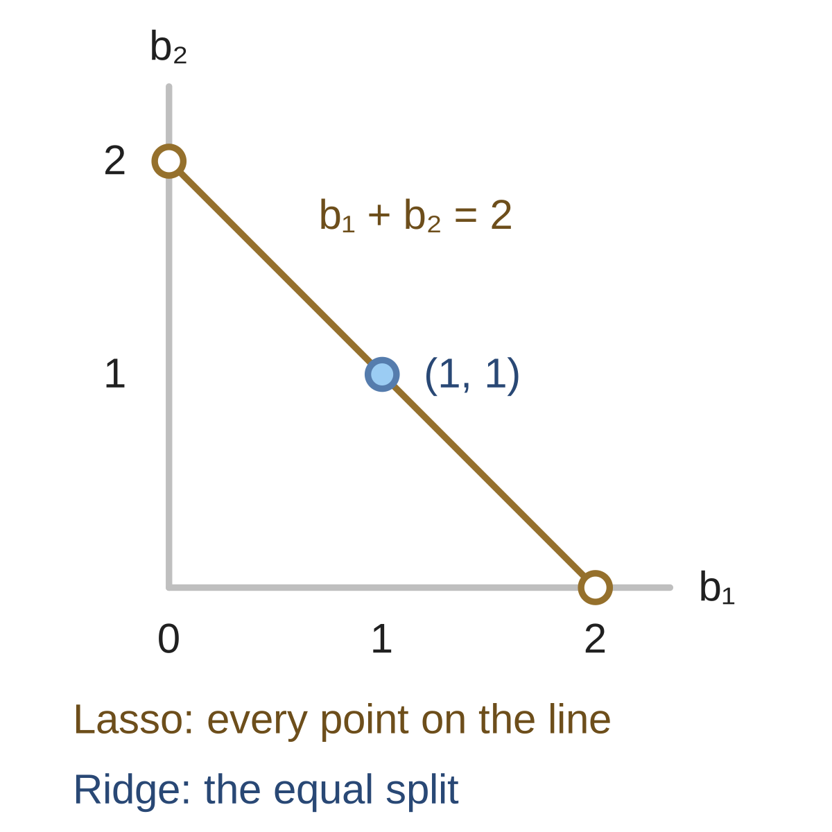
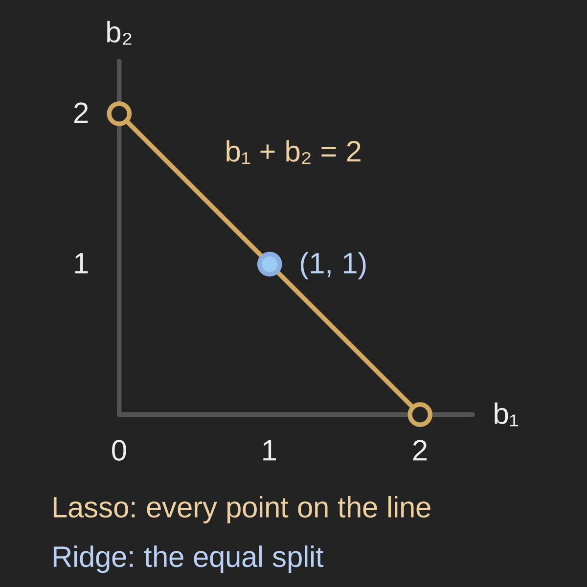
Replace both feature columns by the same centered x with mean square one, and set y = 3x. At λ = 1, every nonnegative pair summing to 2 minimizes the lasso objective. Ridge has the unique solution (1, 1). The blue point is also a lasso optimum; lasso does not require a zero coefficient in this nonunique example.
Analytic duplicate-column example. Lasso objective is ½(3−b₁−b₂)²+|b₁|+|b₂|; ridge replaces that penalty with (b₁²+b₂²)/2.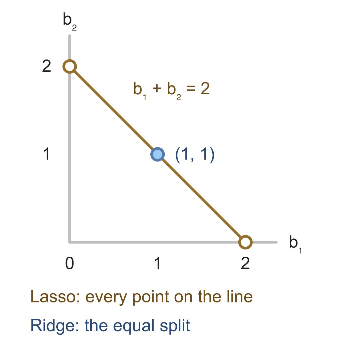
Exact duplication makes the ambiguity visible without numerical noise. With strongly correlated but distinct features, coefficients and the selected subset can be sensitive to changes in the data; perfect duplication is not required for selection to deserve scrutiny. The scikit-learn linear-model guide describes elastic net as a combination of L1 and L2 penalties that is useful with correlated features. It offers another candidate to validate, rather than a guarantee of correct feature discovery.
Choose using validation, scaling, and the model you need
Ridge is a useful baseline when you want shrinkage while keeping contributions from many features. Lasso is worth testing when a sparse model has practical value, such as reducing the number of inputs you must collect. Compare them on validation data appropriate to the task, with a separately chosen penalty for each. A coefficient becoming zero is an optimization result; it is not a statistical significance test or proof of a causal relationship.
Scaling belongs inside that comparison. If a feature is multiplied by , its coefficient can be divided by without changing the prediction. Its absolute-value penalty then becomes times smaller, and its squared penalty becomes times smaller. Leaving such unit differences in place changes which coefficients the penalty makes expensive. StandardScaler is a common way to put varying features on comparable scales, although the right treatment depends on what the inputs mean.
Fit that scaling on training data only. During cross-validation, put preprocessing and the estimator in a pipeline so each fold learns its own scaling; otherwise validation information can leak into training. Keep the test set for the final assessment. The scikit-learn guide to data leakage explains this workflow.
For a numerical look at preprocessing, our normalization and standardization comparison follows one column through both transformations and then transforms an unseen value using the fitted training statistics.
The useful question is whether the resulting predictions, retained inputs, and stability meet your needs. In our four-row example, every zero had an exact mathematical reason. With real data, the same penalty rules apply, but the evidence for choosing a model comes from how it performs beyond the rows that fitted it.
Learn with Glacius
Want to go deeper into the math?
Build your understanding with visual lessons and practice on the concepts from this article.
Check the reasoning
Sources & notes
- scikit-learn: Ridge ↗
Ridge objective, alpha convention, and intercept handling.
- scikit-learn: Lasso ↗
Lasso objective, alpha convention, coordinate descent, and numerical tolerance.
- scikit-learn: linear models ↗
Regularization, correlated predictors, elastic net, and model selection.
- scikit-learn: StandardScaler ↗
Feature scaling before penalized estimation.
- scikit-learn: avoiding data leakage ↗
Fit preprocessing on training data; use pipelines during cross-validation.
Our figures use illustrative mathematical examples unless a dataset is explicitly identified. You can share the original Glacius figures with attribution and a link to this article; linked third-party material retains its own terms.
Keep exploring