Central limit theorem

01The central limit theorem describes the shape of fluctuations in large sums or averages#

The central limit theorem describes the shape of fluctuations in large sums or averages. Under the IID, finite-positive-variance version used here, a properly centered and scaled sum approaches a standard normal distribution. The original observations do not need to look bell-shaped.

The law of large numbers concerns where an average settles. The CLT describes a scale and limiting shape for its deviations. Keep the quantity being approximated clear: a sum and an average have different means and standard deviations.

IID draws have mean $\mu$ and finite positive variance $\sigma^2$. For their sum $S_n$, define:

The CLT gives a standard normal limit as n grows.

A sum of 100 draws with mean 2 and variance 9 has mean 200 and variance 900. The sum’s standard deviation is 30.

Link to this figure ↗Download SVGDownload PNGCopy linkCopy embed

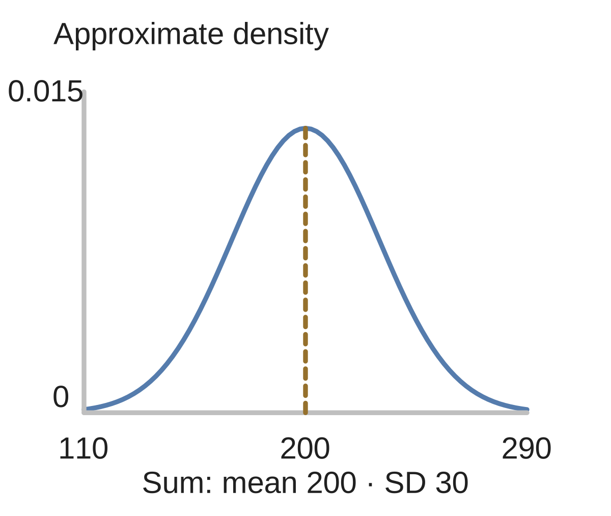
For 100 IID draws with mean 2 and variance 9, the sum has mean $100(2)=200$ and variance $100(9)=900$. Its SD is 30. An observed sum of 230 is $(230-200)/30=1$ standardized unit above its mean. Dividing by 900 would use variance where the standard deviation is required.

02Conditional on using a normal approximation, model the sum by N(nμ,nσ^2)#

Conditional on using a normal approximation, model the sum by $N(n\mu,n\sigma^2)$. The second parameter here is variance.

Subtract the sum’s mean, then divide by its standard deviation. Dividing by n times the individual SD would use the wrong scale.

03The approximation describes a sum or average, not the raw observations#

The approximation describes a sum or average, not the raw observations. Those observations may remain discrete or skewed.

The CLT is asymptotic. It supplies no universal sample size that guarantees a chosen accuracy; inspect those assumptions and accuracy separately.

04This can approximate accumulated independent errors or uncertainty in a sampled average#

This can approximate accumulated independent errors or uncertainty in a sampled average. There is no universal sample-size cutoff that guarantees accuracy for every distribution. Heavy tails, dependence, or an extreme-tail probability can make a simple normal approximation unreliable.