ProbabilityConcept reference

Law of large numbers

For IID finite-variance draws, the sample average converges in probability to the population mean.

2 min read1 figureSources & further reading

On this page 8 sections

Overview
Understand the idea
Chebyshev makes the limit concrete
This is convergence in probability, not a promise that every next average moves closer
Monte Carlo estimates rely on averaging draws from the intended distribution
Key takeaway
Sources & further reading
Concept connections

01Understand the idea#

The law of large numbers describes the stabilization of a sample average around its population expectation under stated assumptions. It explains why collecting more representative independent observations can help estimate an average quantity. It does not say the individual observations become less variable.

The weak law describes sample averages concentrating around their population mean.

Here the draws are IID with finite variance. For any fixed positive error tolerance, the probability that the average misses the mean by at least that tolerance tends to zero.

The average keeps mean $\mu$ , while its variance is $\sigma^2/n$ . More independent draws reduce the variance of the average.

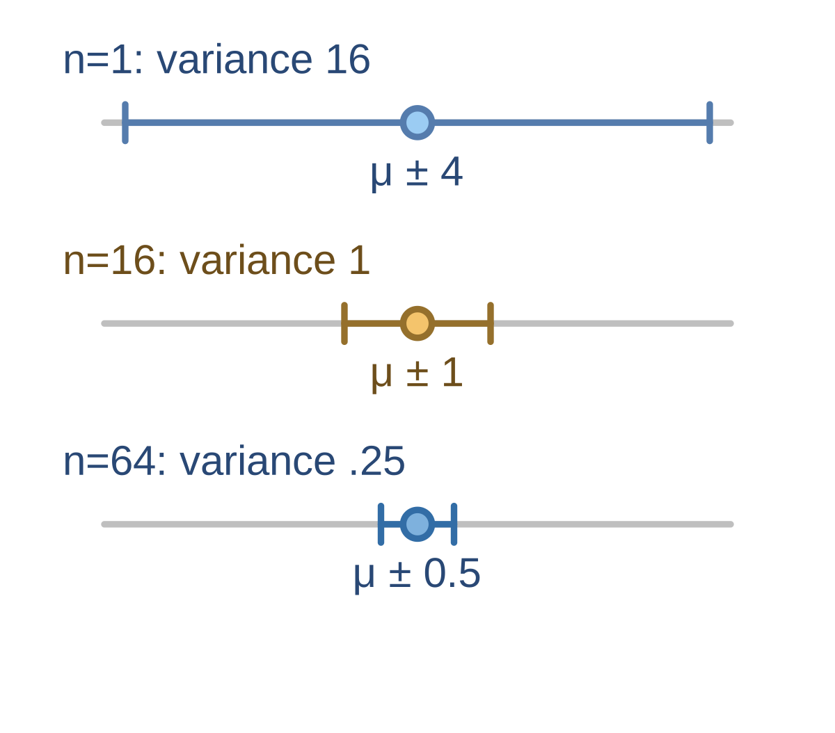
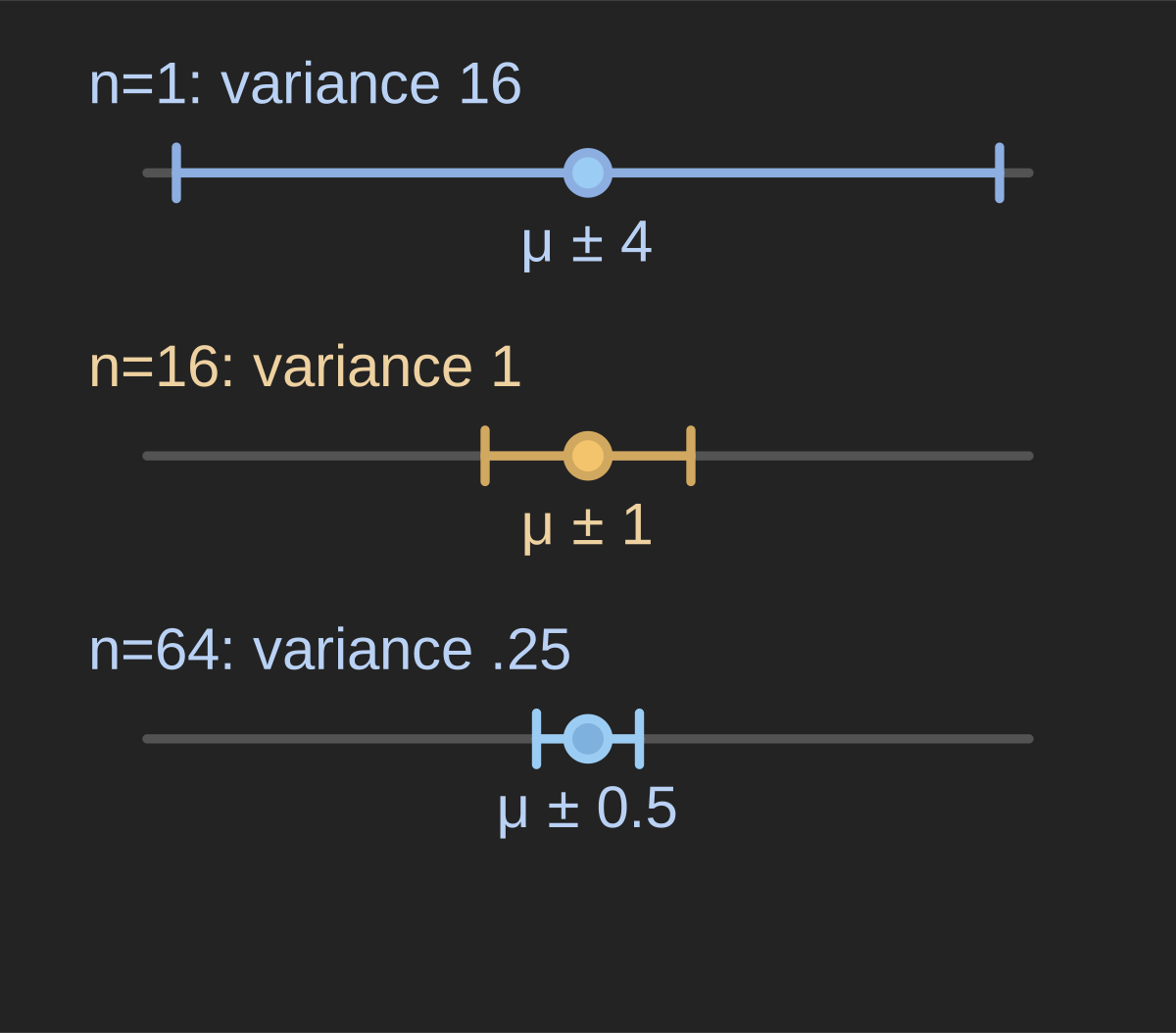
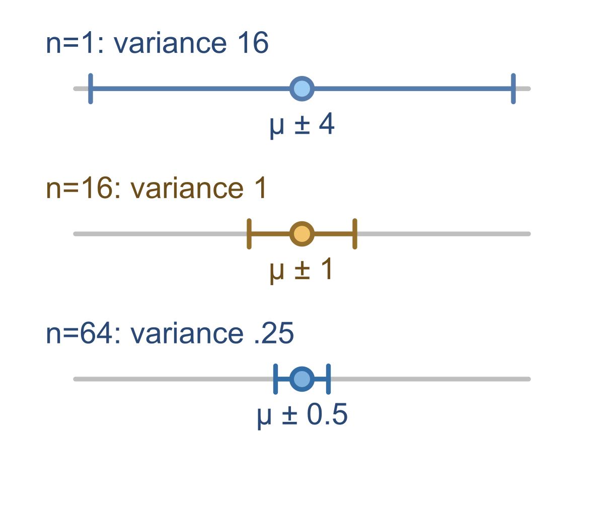
Figure 1IID observations have variance 16. Sample averages at n=16 and n=64 have variances 1 and .25, hence SDs 1 and .5. All centers indicate the same population mean. These are SD spans, not probability intervals or an assumed normal density.

For independent trials with success probability 0.3, encode success as 1 and failure as 0. Their average is the fraction of successes. Ten trials might give 0.5; a larger run might give 0.32. Convergence as sample size grows does not promise a closer estimate at every step.

Check your reasoning

IID draws have mean $4$ and finite variance. As $n\to\infty$ , find $P(3<\bar X_n<5)$ .

A0
B0.5
C1

Show answer and explanation

Mean 4 is inside (3,5), so the probability tends to 1.

02Chebyshev makes the limit concrete#

Chebyshev makes the limit concrete. For fixed $\epsilon>0$ :

\begin{gathered}P(|\bar X_n-\mu|\ge\epsilon)\\\le\frac{\sigma^2}{n\epsilon^2}\end{gathered}

The bound tends to zero as n increases.

Check your reasoning

IID draws have variance $25$ . With $n=100$ , bound $P(|\bar X_n-\mu|\ge 1)$ by Chebyshev, capped at $1$ .

Show answer and explanation

0.25

Average variance is $25/100=0.25$ . Divide by $1^2$ to get upper bound $0.25$ .

03This is convergence in probability, not a promise that every next average moves closer#

This is convergence in probability, not a promise that every next average moves closer. A particular sequence can temporarily move away.

Nor does a large sample shrink each raw observation toward the mean. The concentration belongs to the average.

Check your reasoning

IID, finite variance; fixed $\epsilon>0$ . Draft: the law guarantees $P(|\bar X_n-\mu|\ge\epsilon)=0$ always. Repair.

AAlways zero.
BIt tends to zero.
CAlways one.

Show answer and explanation

It tends to zero.

The limit is zero.

04Monte Carlo estimates rely on averaging draws from the intended distribution#

Monte Carlo estimates rely on averaging draws from the intended distribution. A biased sampling process can stabilize around the wrong population average. More data do not repair a mismatch between the distribution sampled and the quantity you want to estimate.

Key takeaway

Averages concentrate near the mean; individual draws stay variable and each next average need not be closer.

Interpret convergence of an IID sample average under a stated finite-variance assumption.

Sources & further reading

[1]
Pishro-Nik: Law of Large Numbers ↗Pishro-Nik · Article

01Understand the idea#

02Chebyshev makes the limit concrete#

03This is convergence in probability, not a promise that every next average moves closer#

04Monte Carlo estimates rely on averaging draws from the intended distribution#

Averages concentrate near the mean; individual draws stay variable and each next average need not be closer.

Sources & further reading

Reference this concept