Normal probabilities

01Understand the idea#

To find a normal interval probability, convert its endpoints to standard-normal units and compare cumulative areas. A cumulative distribution function gives area to the left, so an interval is the upper cumulative area minus the lower cumulative area.

$\Phi(z)$ is the standard-normal probability to the left of $z$. For $-1<Z<1$, remove the left tail at $-1$ from the left tail at $1$.

Link to this figure ↗Download SVGDownload PNGCopy linkCopy embed

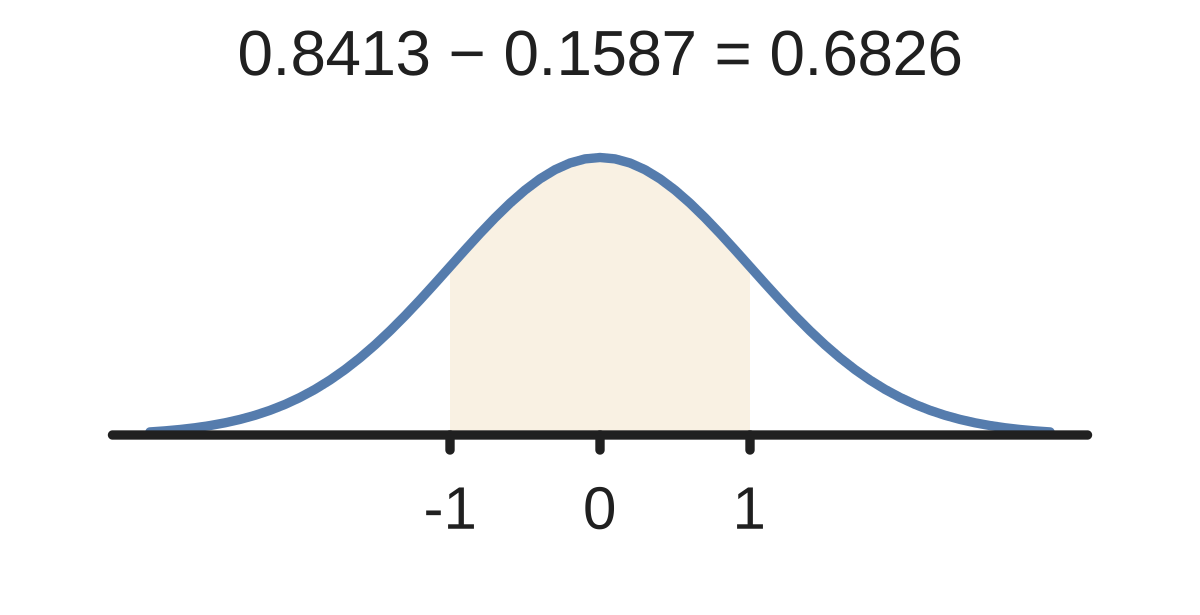
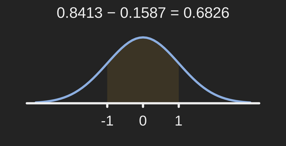
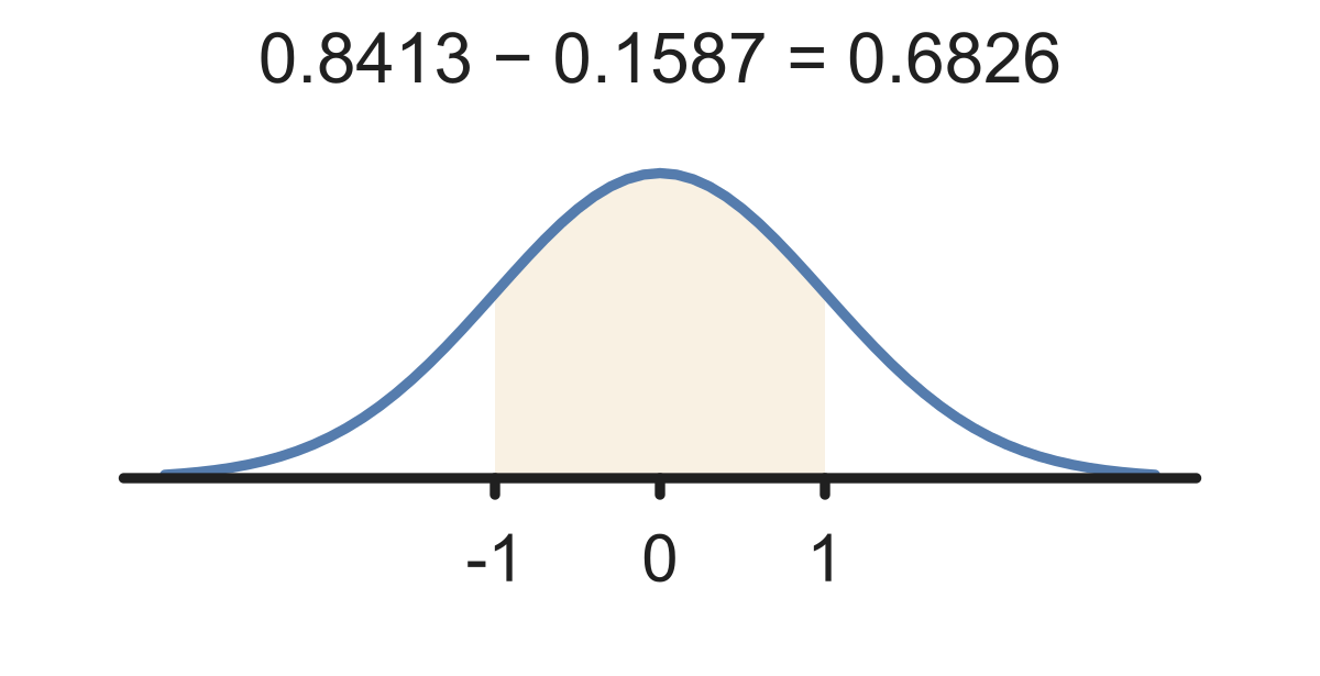
First standardize both raw endpoints using the same mean and SD. Then subtract the lower CDF value from the upper one.

The supplied CDF values are rounded, so the resulting probability is approximate.

For a normal variable with mean 10 and SD 2, the interval $[8,12]$ becomes $[-1,1]$. If supplied values are $\Phi(1)=0.8413$ and $\Phi(-1)=0.1587$, subtract to get 0.6826. The chance above 12 is instead $1-0.8413=0.1587$.

02A right tail is everything beyond a threshold#

A right tail is everything beyond a threshold. Because $\Phi(z)$ counts the left side, the right-tail probability is $1-\Phi(z)$.

03For mean 10, SD 2, and interval 8<X<11, the standard endpoints are -1 and 0.5#

For mean $10$, SD $2$, and interval $8<X<11$, the standard endpoints are $-1$ and $0.5$. With $\Phi(-1)=0.1587$ and $\Phi(0.5)=0.6915$, subtract to get $0.5328$.

04A closer look#

The same procedure can estimate how often a model’s measurement error falls within a stated tolerance. Use a normal approximation only when its assumptions are justified, and retain the accuracy implied by the supplied table values.

Further questions