Grid posteriors
On a finite grid with positive evidence, posterior mass is likelihood times prior mass divided by the sum of all such weights.
On this page 9 sections
- Overview
- A posterior grid keeps uncertainty over an explicitly finite set of parameter candidates
- For prior and likelihood , weights are
- Match candidate labels before multiplying
- Keep candidate labels attached to their masses when lists are reordered
- Key takeaway
- Further questions
- Sources & further reading
- Concept connections
01A posterior grid keeps uncertainty over an explicitly finite set of parameter candidates#
A posterior grid keeps uncertainty over an explicitly finite set of parameter candidates. Each candidate receives a weight from prior mass times likelihood. Normalizing these weights gives a probability distribution you can use for more than selecting a single winner.
Weights total 0.5. Dividing every weight by that same total gives . The posterior keeps all three candidates.
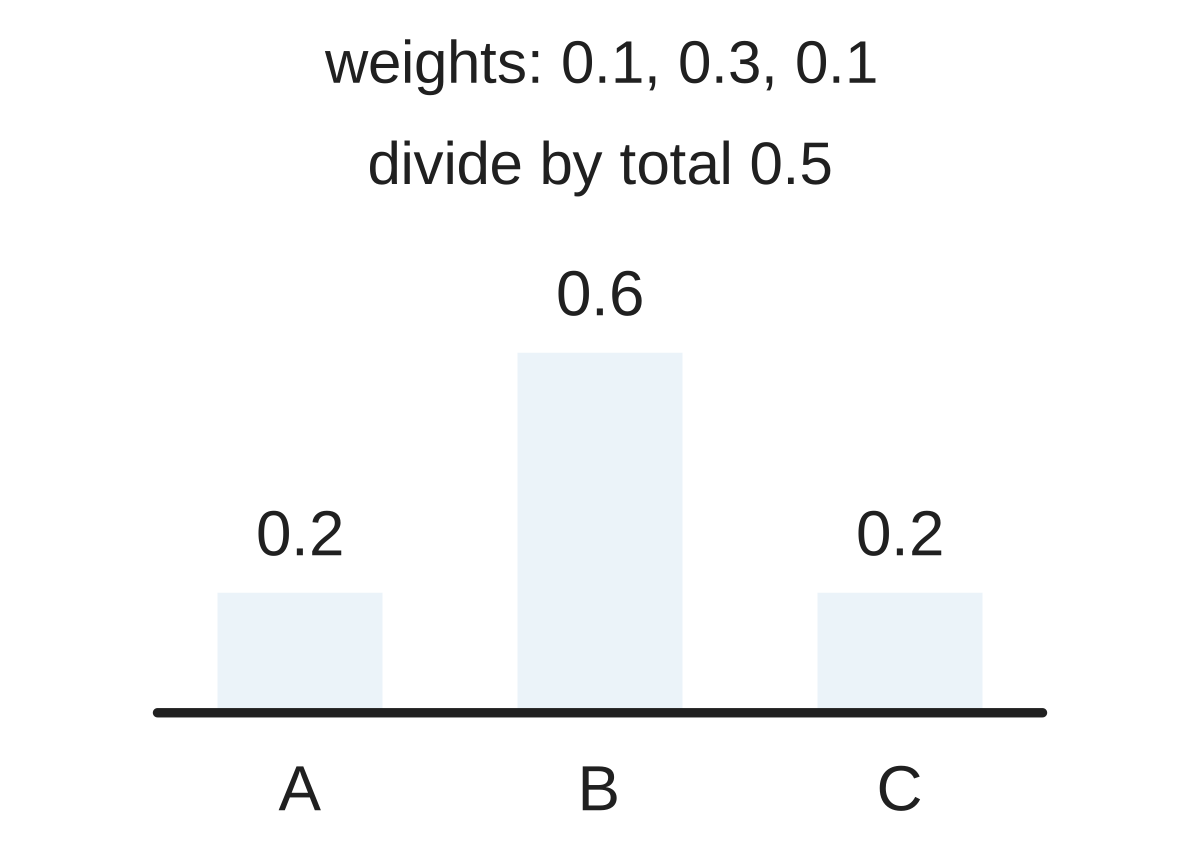
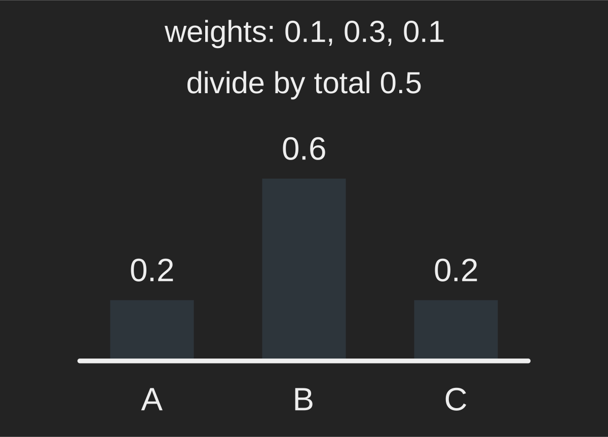
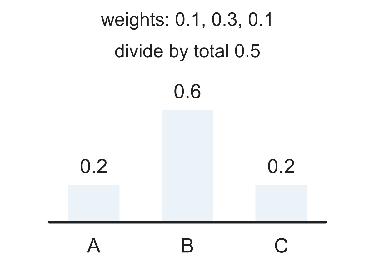
For an explicitly finite grid, multiply each prior mass by its data likelihood. The total of all weights must be positive before normalizing.
For prior and likelihood , weights are . Their sum 0.4 is the normalization constant. Divide both weights by 0.4 to obtain , which sums to 1. Dividing each candidate by a different total would not produce this posterior.
Finite grid (A,B,C). Prior ; likelihood . Give posterior masses in that order.
Show answer and explanation
Divide by total .
02For prior and likelihood , weights are #
For prior and likelihood , weights are . Their total 0.4 gives posterior . Raw weights are not yet a probability distribution.
Finite grid (A,B,C). Prior ; likelihood . Claim: posterior . Repair.
Show answer and explanation
Divide by total .
03Match candidate labels before multiplying#
Match candidate labels before multiplying. Reordering the supplied prior does not change which candidate owns each mass. Zero-weight candidates keep mass 0; divide every other weight by the same positive total.
Prior for (C,B,A) is . Data likelihood for (A,B,C) is . Return posterior (A,B,C).
Show answer and explanation
Divide by total .
04Keep candidate labels attached to their masses when lists are reordered#
Keep candidate labels attached to their masses when lists are reordered. This posterior expresses uncertainty within the finite model; omitted parameter values receive no probability. Approximating a continuous model with a grid requires additional care in assigning prior mass.
Multiply matching likelihoods and priors, then divide every weight by their positive total. Keep the complete ordered distribution.
- Normalize posterior weights over a finite parameter grid.
Further questions
What if every candidate has zero weight?
Sources & further reading
- [1]Pishro-Nik, §1.4.3 Bayes’ Rule ↗Textbook · Book
- [2]