P-values
A p-value is the null-model probability of a statistic at least as extreme as observed under a stated rule.
On this page 8 sections
01Understand the idea#
A p-value measures how often the null model would produce a test statistic at least as extreme as the observed one, using the test’s specified direction. It asks about possible data under a model. It does not give the probability that the null model is true.
A p-value is a probability calculated under a specified null model. Sum the probabilities of statistic values at least as extreme as the observation, using the stated tail rule. For discrete values, “at least” includes ties.
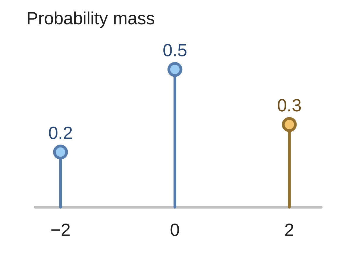
This null law assigns masses 0.2, 0.5, 0.3 to T=−2,0,2. Observed t=2 and the rule T≥t select only T=2. Its null probability is 0.3.
For an upper-tail test, suppose a null model gives probabilities 0.7, 0.2, and 0.1 to statistics 0, 1, and 2. Observing 1 includes both 1 and the more extreme 2, so the p-value is . Using only the observed statistic’s mass would omit more extreme outcomes.
Null masses T: -2:0.2, -1:0.3, 1:0.1, 2:0.4. Observed t=-2. Tail |T|≥|t|. p-value?
Show answer and explanation
Included mass: 0.2 + 0.4 = 0.6.
02An absolute-tail rule selects either sign#
An absolute-tail rule selects either sign. With masses 0.1,0.2,0.4,0.3 at T=−3,−1,0,2, observed t=−2 selects −3 and 2. Their mass is 0.4. The tails are asymmetric, so doubling one tail would give the wrong answer.
A CDF gives F(t)=P(T≤t). For a continuous null model, there is no mass exactly at t. A lower-tail p-value is F(t); an upper-tail p-value is 1−F(t). For F(1)=0.9, the upper tail is 0.1.
Continuous null CDF: F(3)=0.96. Observed t=3. Tail T≥t. p-value?
Show answer and explanation
1−F(t) = 0.04.
03The tail can have probability 0 or 1 under a supplied model#
The tail can have probability 0 or 1 under a supplied model. Even a small p-value does not assign a probability to H0 being true. It describes how often the stated statistic tail occurs if that null model generates the data.
Null masses T: 0:0.6, 1:0.25, 2:0.15. Observed t=1. Tail T≥t. “Probability H0 is true.” Repair value / meaning.
Show answer and explanation
0.25+0.15=0.4.
04A closer look#
When comparing a model improvement with a no-improvement null, report the effect estimate and uncertainty along with the p-value. A small p-value need not mean the effect is practically large, and a large p-value does not establish exact equality or prove the null.
Use the supplied null law and tail rule, include tied discrete values, and sum their probabilities.
- Compute the stated null tail probability.
Sources & further reading
- [1]
- [2]American Statistical Association, 2016 Statement on Statistical Significance and P-Values ↗American Statistical Association · Article