ProbabilityConcept reference

Bayes' rule

Bayes’ rule expresses the probability of a hypothesis given positive-probability evidence as their joint probability divided by the evidence probability.

2 min read1 figureSources & further reading

On this page 8 sections

Overview
Change the reference group
Prior, likelihood, posterior
See the denominator directly
Read the update
Key takeaway
Sources & further reading
Concept connections

01Change the reference group#

Bayes' rule answers how plausible a hypothesis is after observing evidence. It reverses a conditional probability by carefully changing the reference group. The chance of evidence within a hypothesis need not equal the chance of that hypothesis within the evidence.

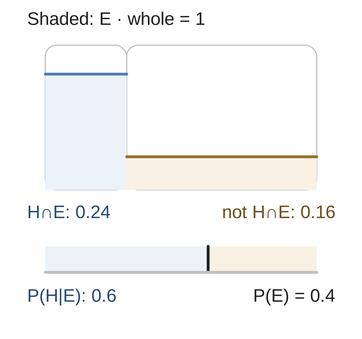
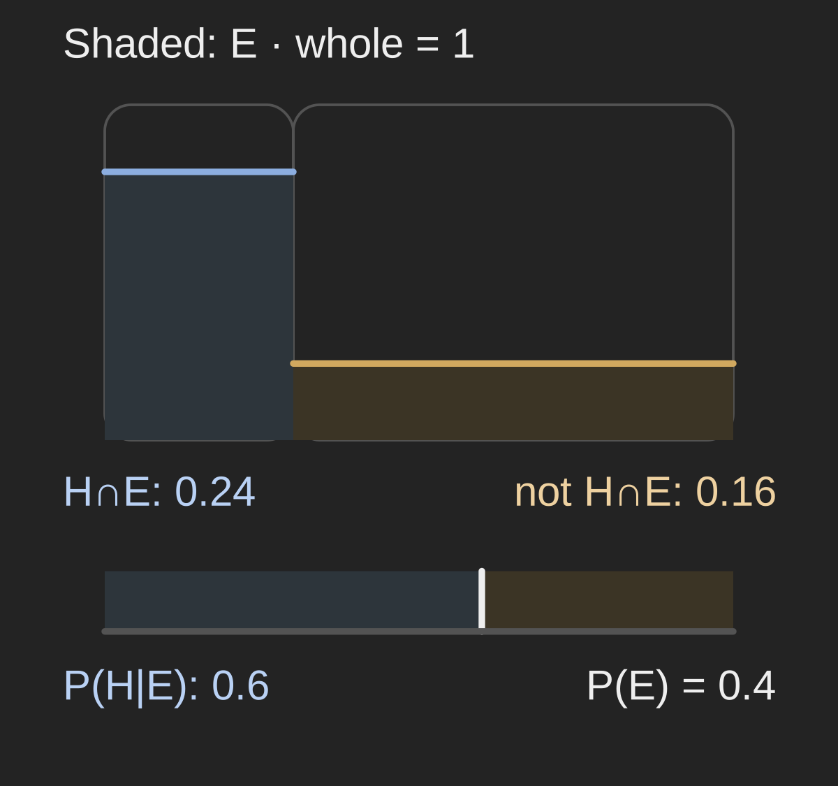
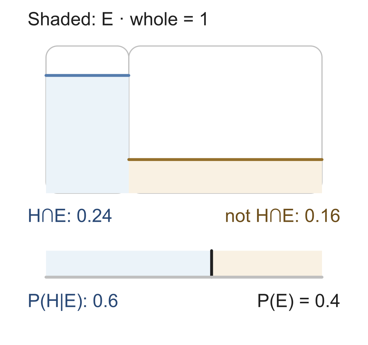
Write $H$ for the hypothesis and $E$ for the evidence. If $P(H)=0.3$ and $P(E\mid H)=0.8$ , then the joint probability is $0.3(0.8)=0.24$ . This is the share satisfying both conditions.

If $P(E)=0.4$ , that joint share occupies $0.24/0.4=0.6$ of the evidence group. Dividing by the evidence probability makes the whole evidence group the new denominator.

Figure 1P(H)=.3 and P(E|H)=.8 give joint area .24. The remaining evidence is .16 in not-H, so its conditional E rate is .16/.7. E has total .4. The lower evidence-only strip has H share .24/.4=.6.

Link to this figure ↗Download SVG Download PNG

02Prior, likelihood, posterior#

The multiplication rule gives $P(H\cap E)=P(H)P(E\mid H)$ . The definition of conditioning then gives

\begin{gathered}P(H\mid E)\\=\frac{P(H)P(E\mid H)}{P(E)}\end{gathered}

The prior $P(H)$ describes the hypothesis before this evidence. The likelihood $P(E\mid H)$ measures how probable the evidence would be under it. The posterior $P(H\mid E)$ describes the hypothesis within the observed evidence group.

Check your reasoning

P(H)=0.4, P(E | H)=0.5, P(E)=0.25. Find P(H | E).

Show answer and explanation

0.8

0.2 / 0.25 = 0.8.

03See the denominator directly#

In 1000 records, 100 satisfy a hypothesis and 90 of those show the evidence. If 300 records show evidence overall, the posterior is $90/300=0.3$ . The evidence rate within the hypothesis is $90/100=0.9$ . The numerators match; the reference groups differ.

Check your reasoning

Among 200 uniform records, 50 have H. Within H, the E rate is 0.4. Exactly 40 records have E. Find P(H | E).

Show answer and explanation

0.5

20 H-and-E records out of 40: 0.5.

All routes to the evidence belong in $P(E)$ , including evidence without $H$ . Computing this total from a partition uses the earlier total-probability rule. A posterior above one flags inconsistent supplied probabilities or a calculation error.

04Read the update#

If $P(E\mid H)=P(E)>0$ , the factors cancel and the posterior equals the prior. The evidence does not change this hypothesis's probability. A zero likelihood gives posterior zero when total evidence is positive.

Check your reasoning

P(H)=0.25, P(E | H)=0.8, P(E)=0.5. “P(H | E)=0.8.” Repair it.

A0.8
B0.4
C0.2

Show answer and explanation

0.4

Joint 0.2; divide by 0.5: 0.4.

When $P(E)=0$ , this finite-event ratio is undefined. Within its stated assumptions, Bayes' rule combines prior probability with evidence fit. It does not let a high likelihood erase a very small prior automatically.

Key takeaway

Multiply prior by likelihood, then divide by all evidence. The two conditional directions use different denominators.

Reverse a conditional using the full evidence total.

Sources & further reading

[1]
Pishro-Nik, Introduction to Probability: 1.4.3 Bayes Rule ↗www.probabilitycourse.com · Article
[2]
Dive into Deep Learning, §2.6 Probability and Statistics ↗d2l.ai · Article

01Change the reference group#

02Prior, likelihood, posterior#

03See the denominator directly#

04Read the update#

Multiply prior by likelihood, then divide by all evidence. The two conditional directions use different denominators.

Sources & further reading

Reference this concept