Discrete likelihoods
A discrete likelihood evaluates the fixed sample joint PMF as a function of the candidate parameter. Independent factors multiply.
On this page 9 sections
01Understand the idea#
Likelihood compares candidate parameter settings by how much probability they assign to the data that actually occurred. The data stay fixed while the candidate changes. This is the direction used when fitting a probabilistic model.
Keep the observed sequence fixed at . Candidate assigns factors . Independence makes their product .
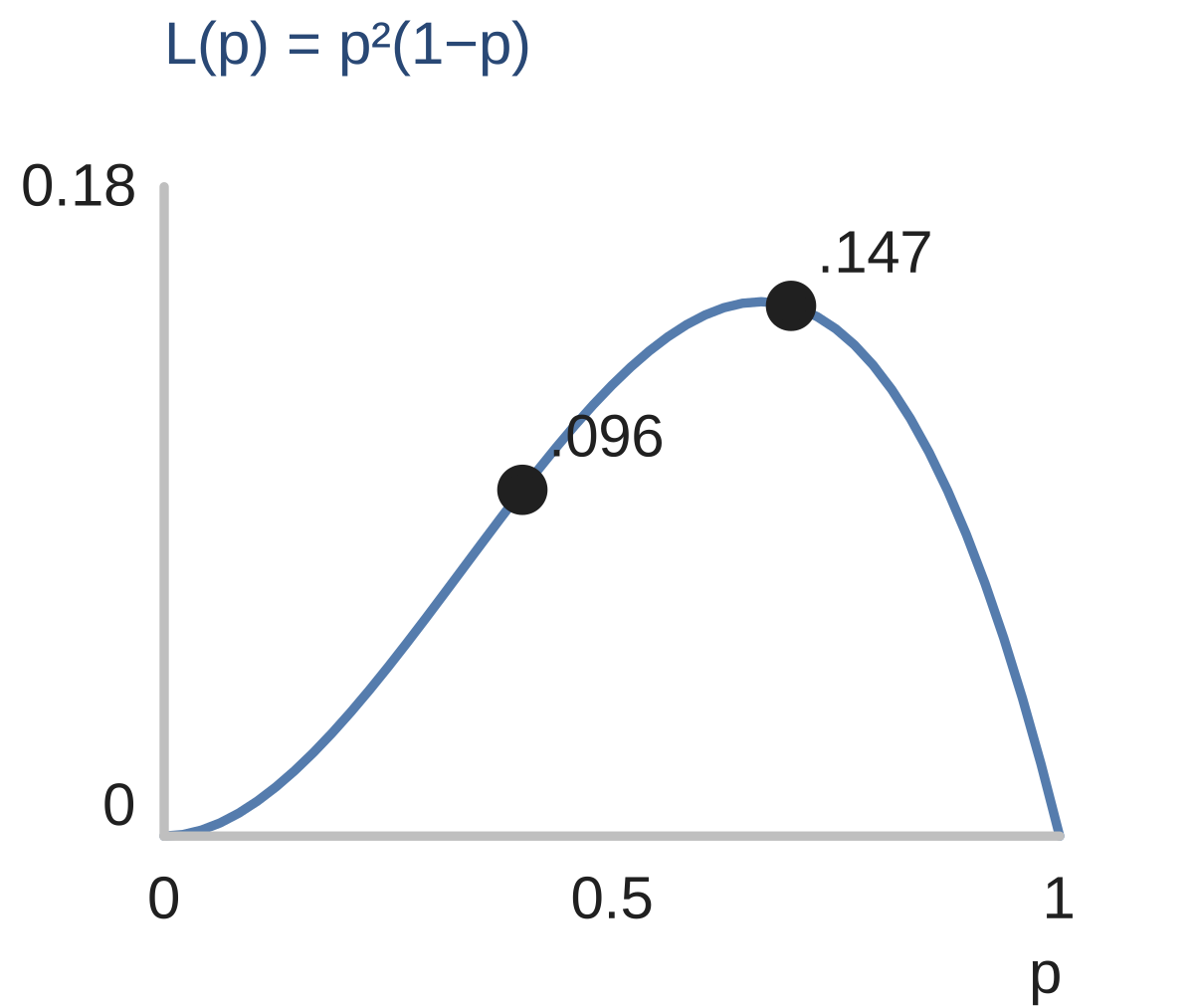
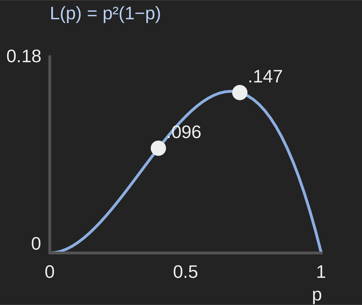
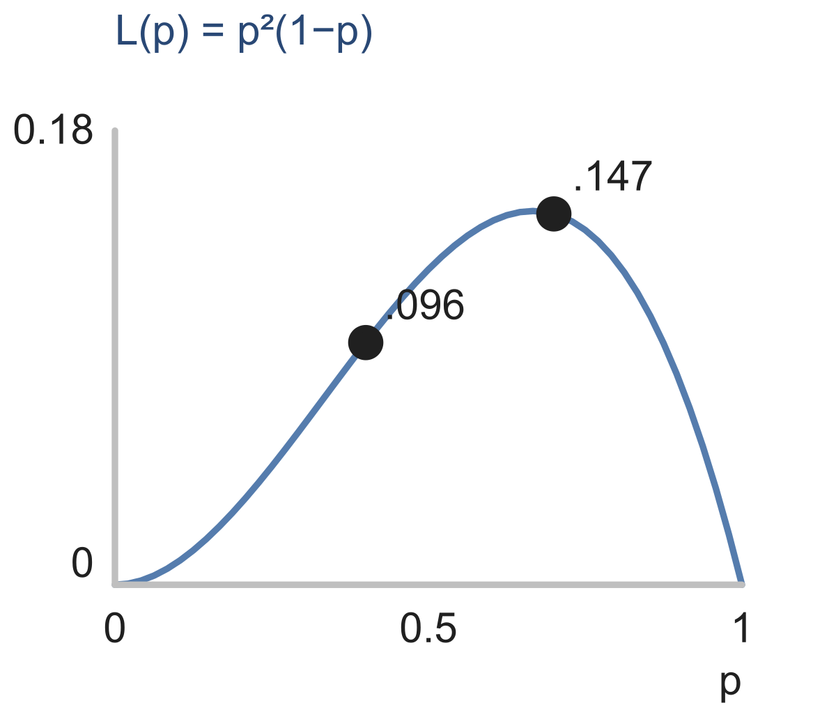
Likelihood is the sample probability viewed as a function of the candidate parameter. For independent observations, multiply the probability of every observed value.
For an ordered independent binary sample and candidate success probability 0.4, the factors are . Multiply to get . Candidate 0.7 instead gives . The same observations favor the second candidate by likelihood.
Ordered iid Bernoulli sample , . Give its likelihood.
Show answer and explanation
.
02For the ordered sample at , use #
For the ordered sample at , use . Adding the factors would give 1, which is not the probability of both observations. An ordered sequence also needs no count-combination factor.
Ordered iid Bernoulli sample , . Reported by adding factors. Repair.
Show answer and explanation
.
03For categorical data, use the observed label to select each factor from the candidate PMF#
For categorical data, use the observed label to select each factor from the candidate PMF. Repeated labels contribute repeated factors. Compare candidates on the same complete sample; their likelihoods need not sum to 1.
Ordered iid . PMFs on : A ; B . ?
Show answer and explanation
A: ; B: .
04These likelihoods do not need to sum to 1 across candidates#
These likelihoods do not need to sum to 1 across candidates. They are probabilities of the fixed sample under separate models, not posterior probabilities of the models. Adding a prior and normalizing is a later Bayesian step. The ordered sequence here also differs from the event “two successes in any order.”
For fixed ordered independent data, multiply observation probabilities under each candidate. Likelihood is not posterior probability.
- Evaluate candidate parameters using a fixed discrete sample's probability model.
Further questions
What changes when the observations are continuous?
Sources & further reading
- [1]Pishro-Nik, §8.2.3 Maximum Likelihood Estimation ↗Textbook · Book