Sampling distributions
A sampling distribution is the probability distribution of an estimator under a fixed sampling scheme.
On this page 8 sections
01Understand the idea#
A sampling distribution describes the values a statistic would take across repeated samples generated by the same sampling process. It is a distribution of estimates, not a histogram of the original observations in one sample.
Imagine repeatedly drawing the same number of records and computing a mean each time. Each sample contributes one mean to the sampling distribution. Its spread measures how much the estimate would change if the sample were collected again.
A sampling distribution describes the outputs of an estimator across repeated samples. Keep the sampling scheme, sample size and rule fixed. Record one output per sample, rather than pooling its raw observations.
Suppose each have probability . For , their outputs are .
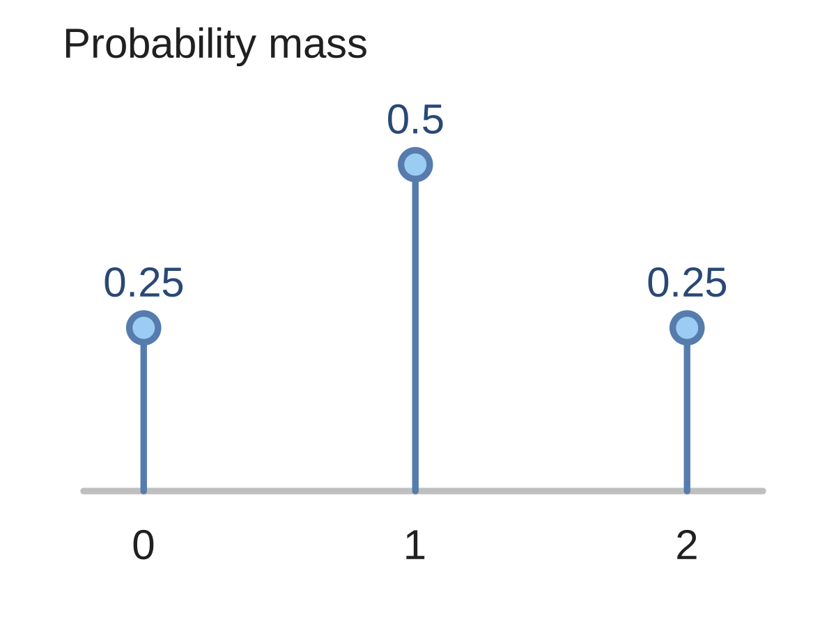
Take two independent draws from a population equally likely to return 0 or 2. The ordered pairs each have probability . Their means are . Combine samples with the same mean: the probabilities at 0, 1, 2 are .
Both middle samples give . Add their probabilities: . Thus the masses at are . Distinct outputs need not be equally likely.
All pairs (x,y): (0,0):1/4; (0,4):1/4; (4,0):1/4; (4,4):1/4. T=max(x,y). Masses at 0,4?
Show answer and explanation
P(T=0)=1/4; P(T=4)=3/4.
02For a largest-reading rule, record the largest value in each new sample#
For a largest-reading rule, record the largest value in each new sample. For a count rule, record that count. A histogram of all the individual readings describes a different variable.
Same random scheme: 5 readings. Rule: count readings above 10. Record what across samples?
Show answer and explanation
Keep the count.
03Some tasks list unequal sample probabilities#
Some tasks list unequal sample probabilities. Use those masses when combining outputs. The notation means that complete pair has probability . The displayed list is exhaustive.
All pairs (x,y): (0,0):1/4; (0,2):1/2; (2,2):1/4. T=x+y. Masses at 0,2,4? “Distinct outputs get equal masses.”
Show answer and explanation
Masses: 1/4, 1/2, 1/4.
04Uncertainty intervals and standard errors concern this across-sample variation#
Uncertainty intervals and standard errors concern this across-sample variation. Observing many different values within one dataset is a different source of spread. Keep the sampling rule and sample size fixed when describing one sampling distribution.
Evaluate the same rule on each possible sample and combine the probabilities of equal outputs.
- Map repeated samples to estimator-output probabilities.
Sources & further reading
- [1]University of Illinois, Data Science Exploration: Sampling Distributions ↗University of Illinois · Article
- [2]Pishro-Nik, Introduction to Probability, 8.1.1 Random Sampling ↗Pishro-Nik, Introduction to Probability · Book